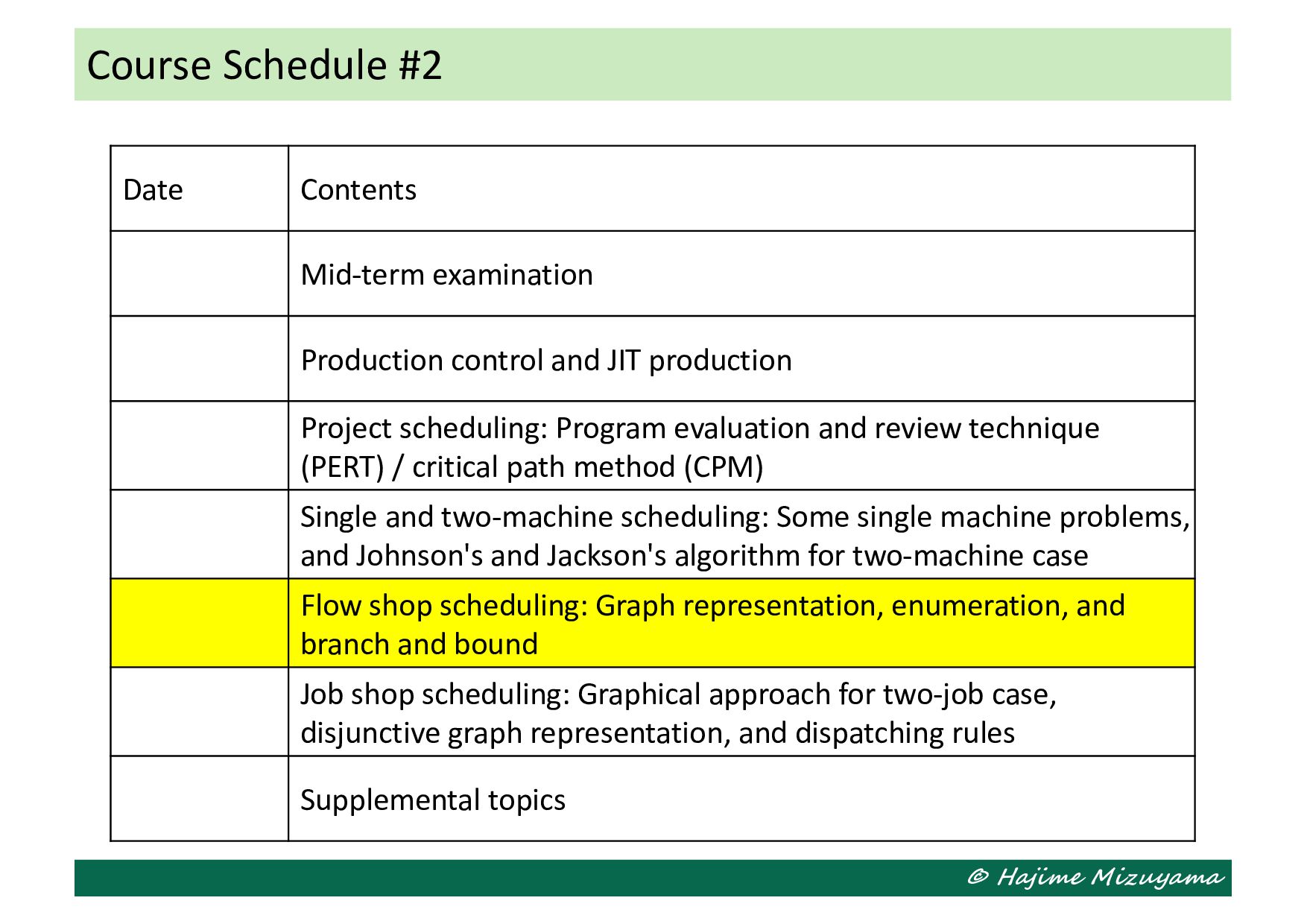
Production control and JIT production Project scheduling: Program evaluation and review technique (PERT) / critical path method (CPM) Single and two-machine scheduling: Some single machine problems, and Johnson's and Jackson's algorithm for two-machine case Flow shop scheduling: Graph representation, enumeration, and branch and bound Job shop scheduling: Graphical approach for two-job case, disjunctive graph representation, and dispatching rules Supplemental topics
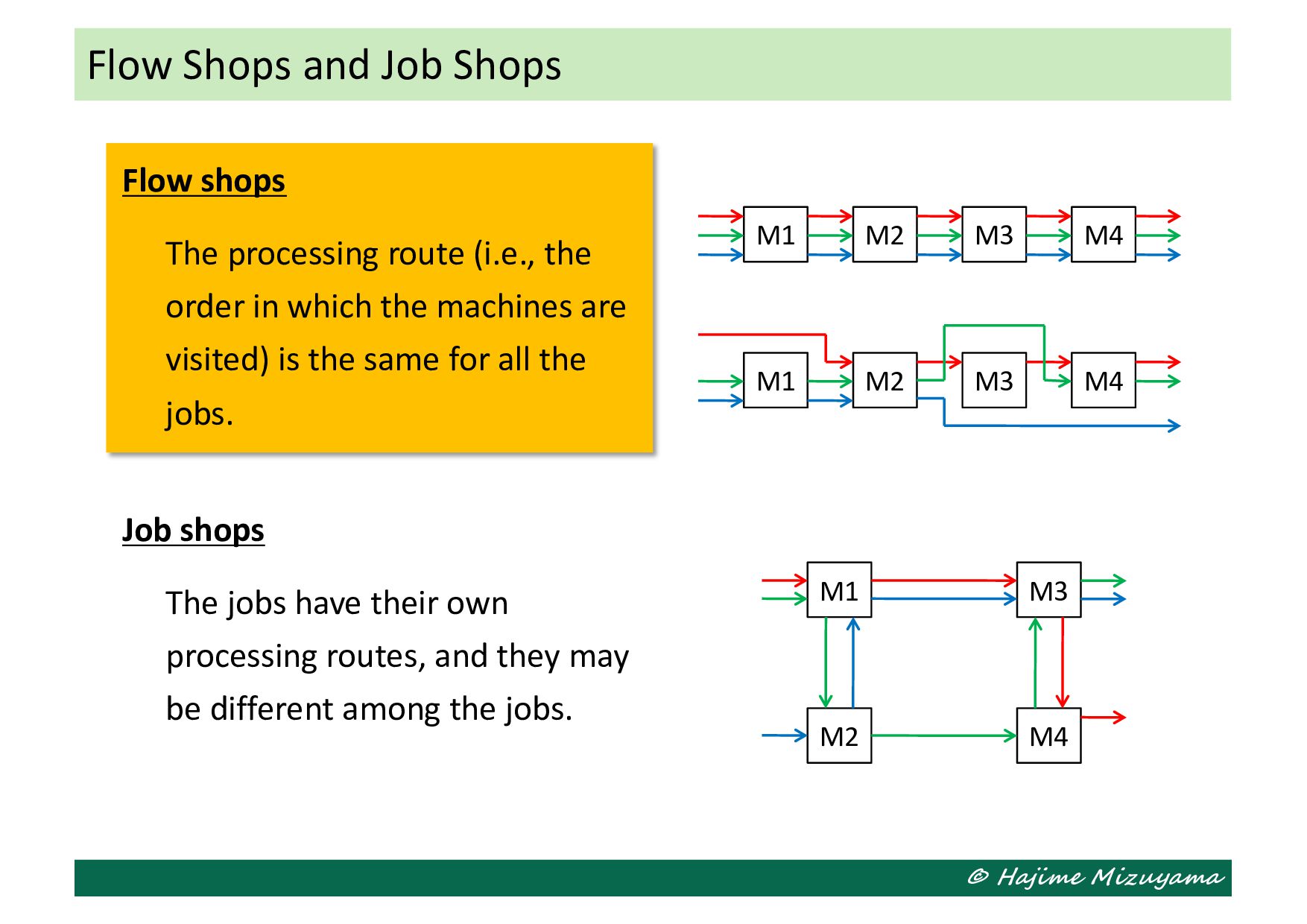
The processing route (i.e., the order in which the machines are visited) is the same for all the jobs. Job shops The jobs have their own processing routes, and they may be different among the jobs. M1 M2 M3 M4 M1 M2 M3 M4 M1 M2 M3 M4
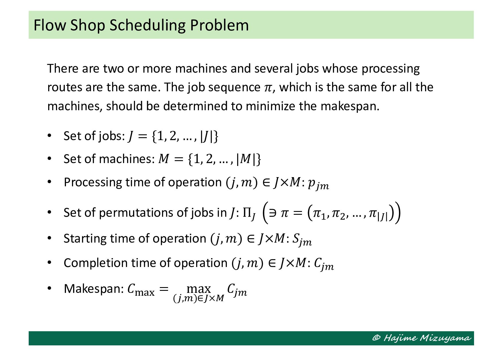
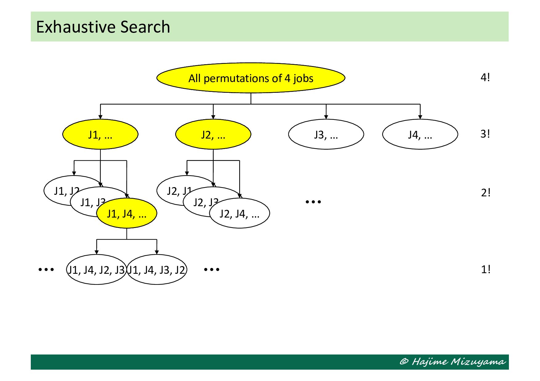
several jobs whose processing routes are the same. The job sequence 𝜋, which is the same for all the machines, should be determined to minimize the makespan. • Set of jobs: 𝐽 = {1, 2, … , |𝐽|} • Set of machines: 𝑀 = {1, 2, … , |𝑀|} • Processing time of operation (𝑗, 𝑚) ∈ 𝐽×𝑀: 𝑝!" • Set of permutations of jobs in 𝐽: Π# ∋ 𝜋 = 𝜋$ , 𝜋% , … , 𝜋 # • Starting time of operation (𝑗, 𝑚) ∈ 𝐽×𝑀: 𝑆!" • Completion time of operation (𝑗, 𝑚) ∈ 𝐽×𝑀: 𝐶!" • Makespan: 𝐶&'( = max (!,")∈#×. 𝐶!" Flow Shop Scheduling Problem
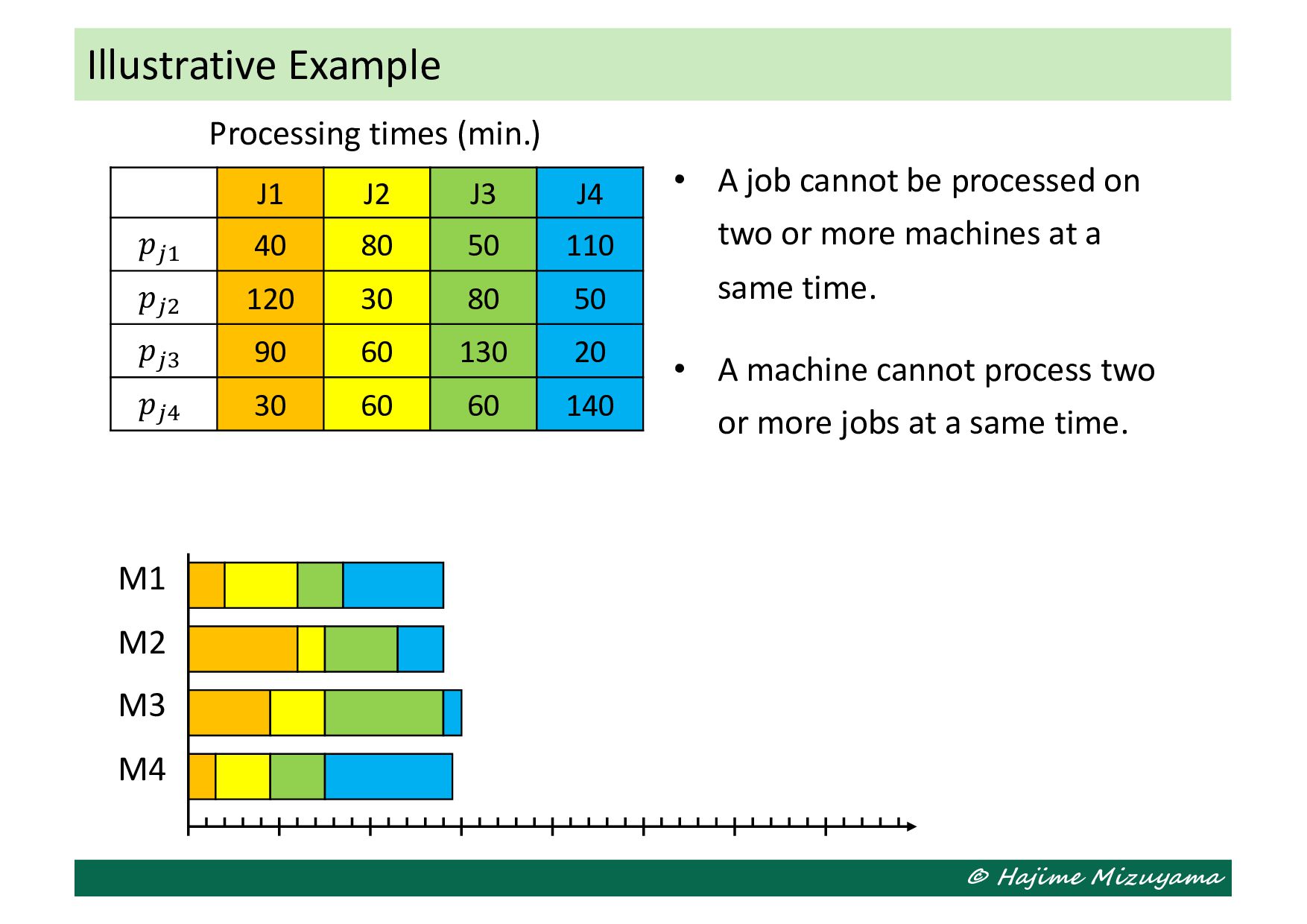
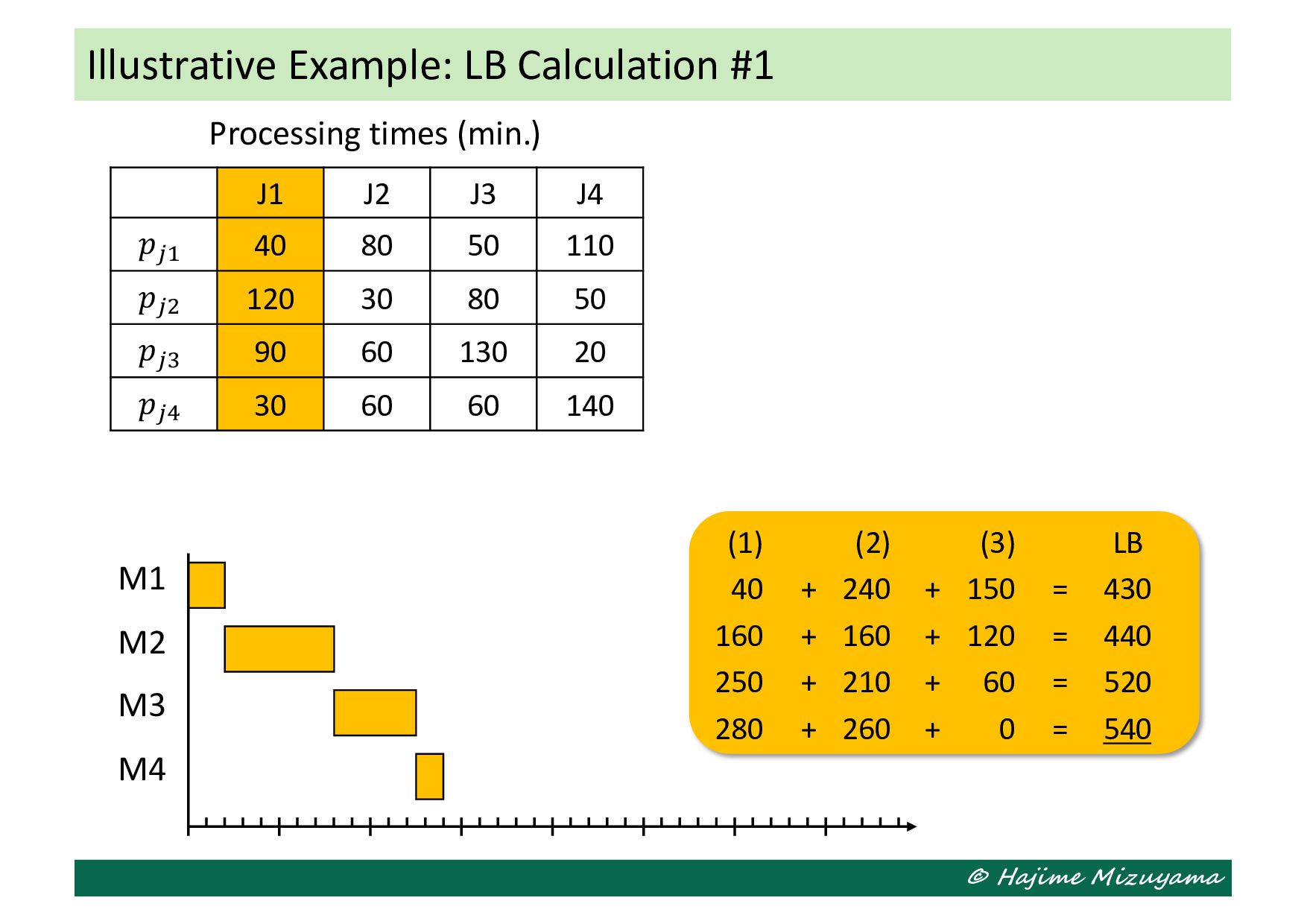
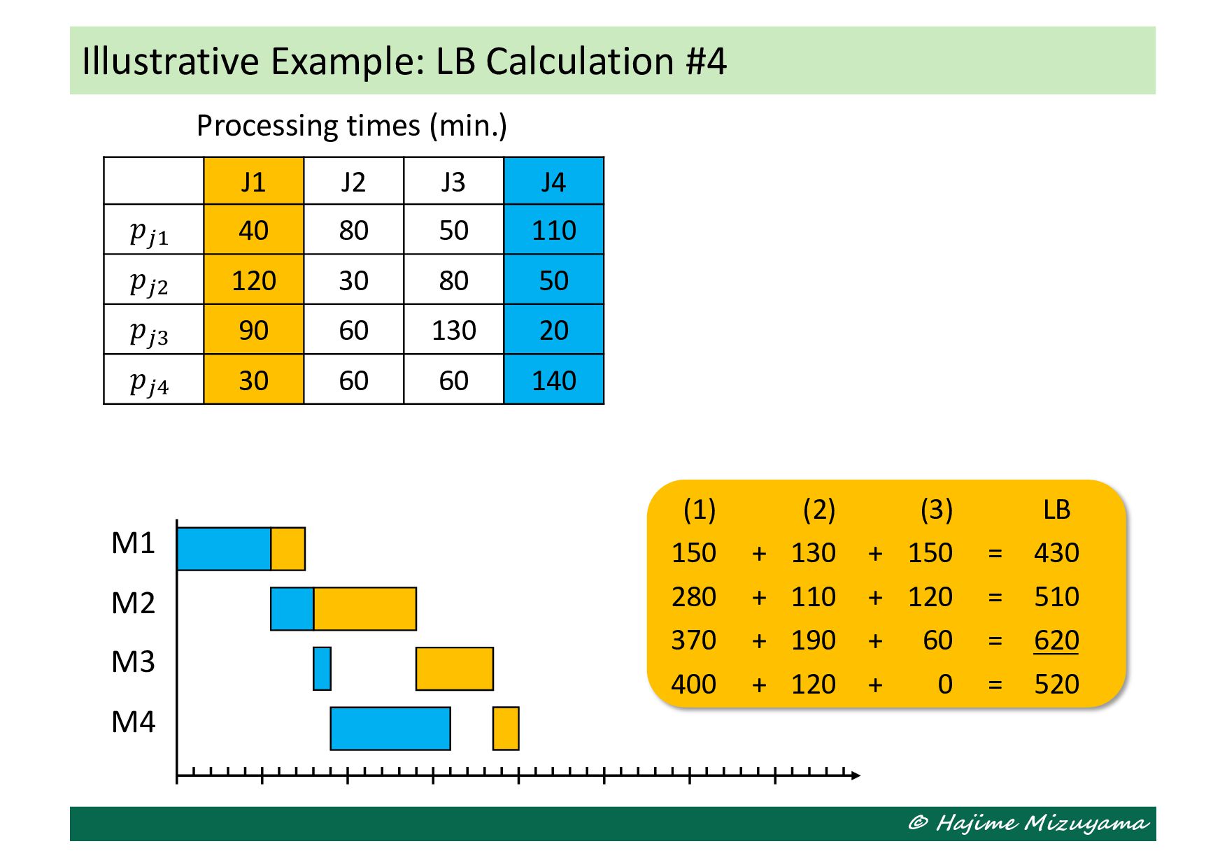
processed on two or more machines at a same time. • A machine cannot process two or more jobs at a same time. J1 J2 J3 J4 𝑝!" 40 80 50 110 𝑝!# 120 30 80 50 𝑝!$ 90 60 130 20 𝑝!% 30 60 60 140 Processing times (min.) M1 M2 M3 M4
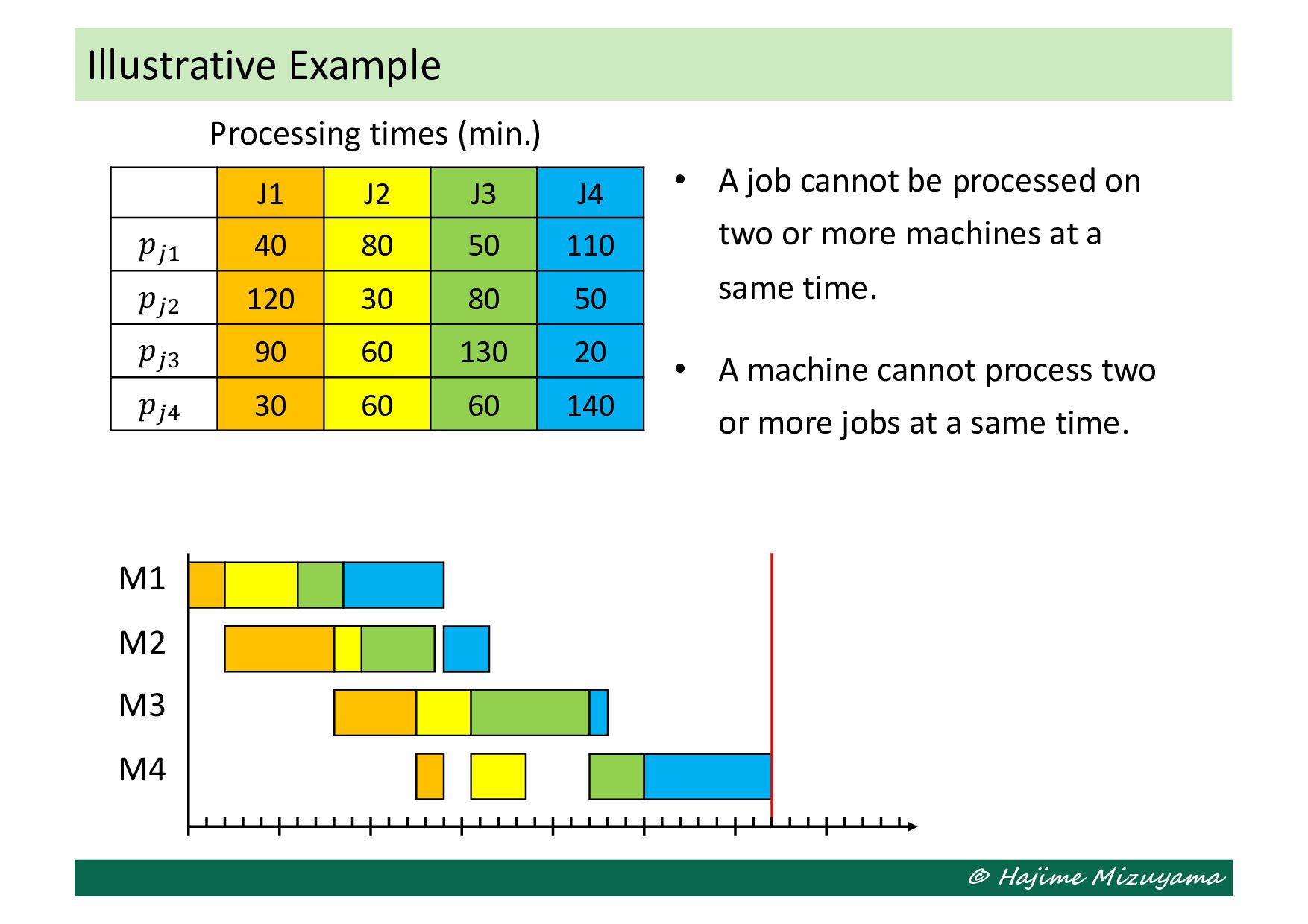
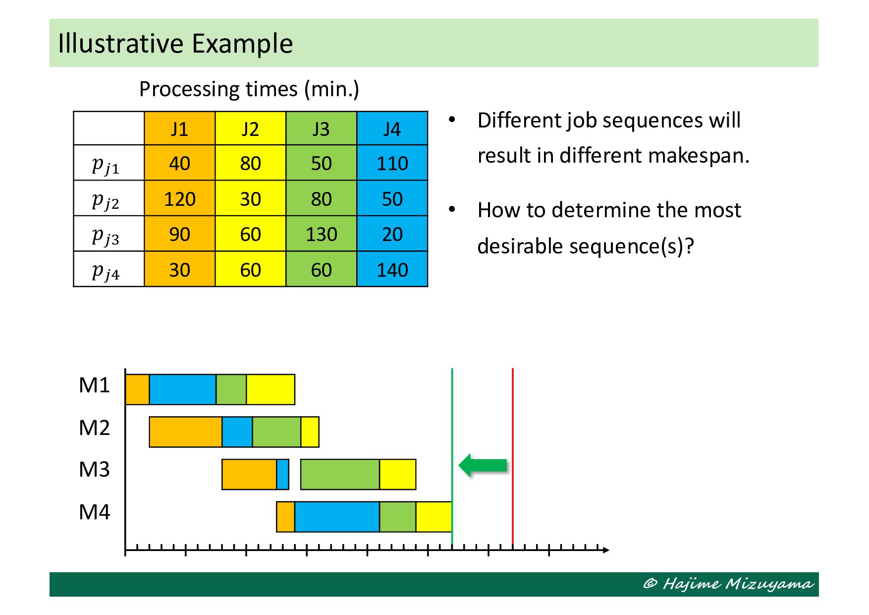
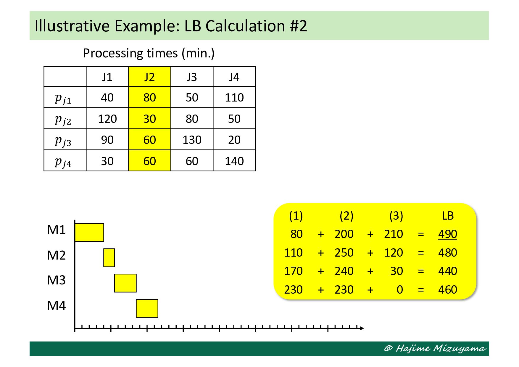
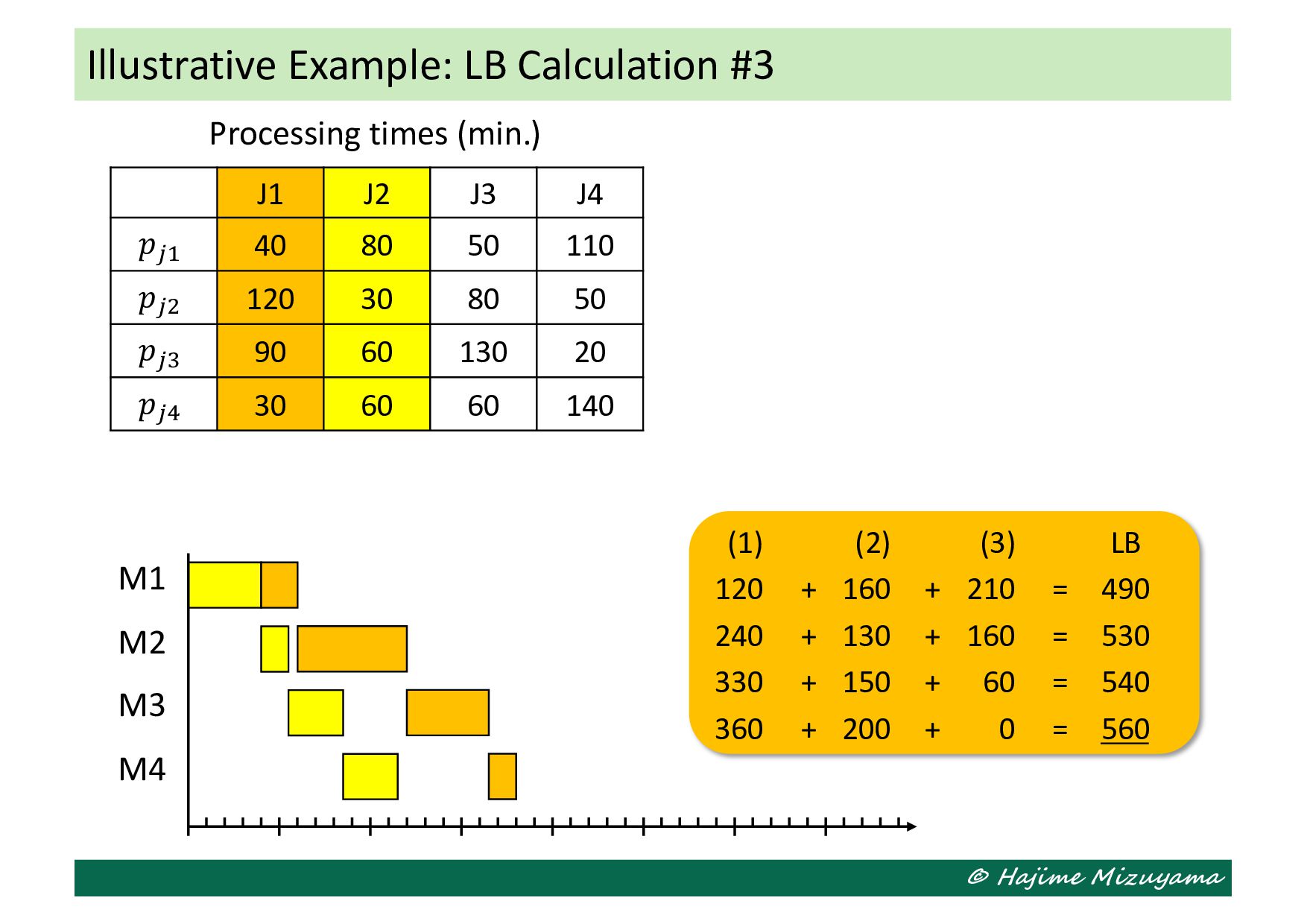
processed on two or more machines at a same time. • A machine cannot process two or more jobs at a same time. J1 J2 J3 J4 𝑝!" 40 80 50 110 𝑝!# 120 30 80 50 𝑝!$ 90 60 130 20 𝑝!% 30 60 60 140 Processing times (min.) M1 M2 M3 M4
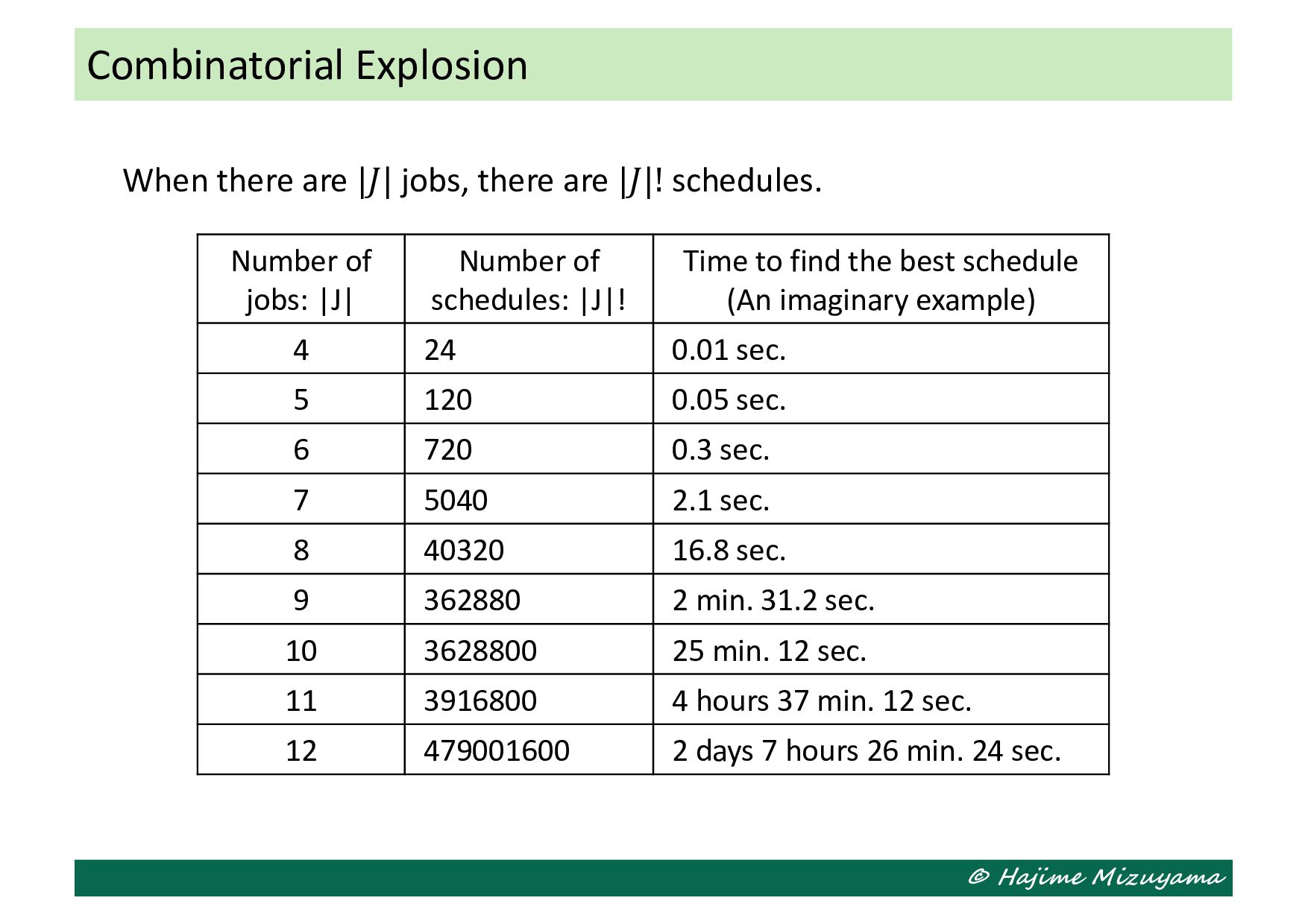
|𝐽|! schedules. Combinatorial Explosion Number of jobs: |J| Number of schedules: |J|! Time to find the best schedule (An imaginary example) 4 24 0.01 sec. 5 120 0.05 sec. 6 720 0.3 sec. 7 5040 2.1 sec. 8 40320 16.8 sec. 9 362880 2 min. 31.2 sec. 10 3628800 25 min. 12 sec. 11 3916800 4 hours 37 min. 12 sec. 12 479001600 2 days 7 hours 26 min. 24 sec.
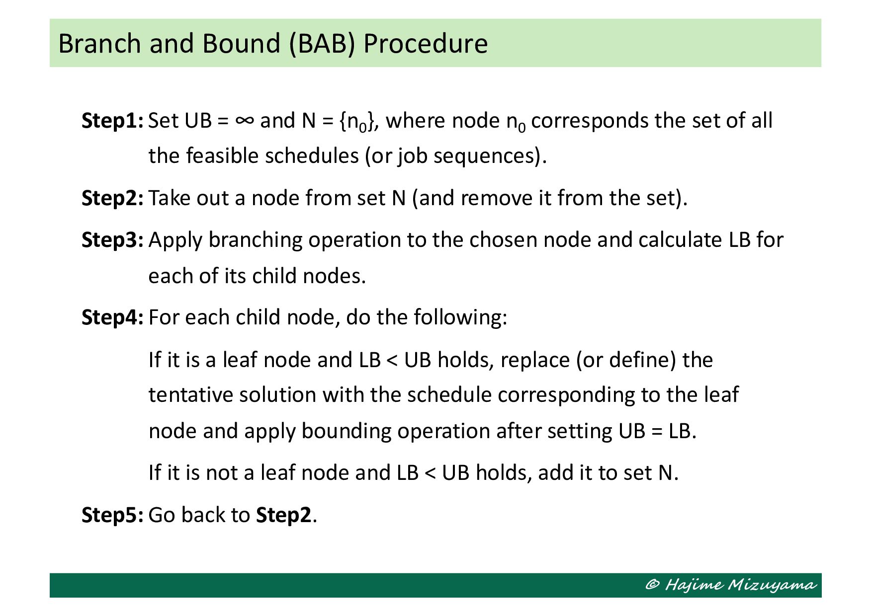
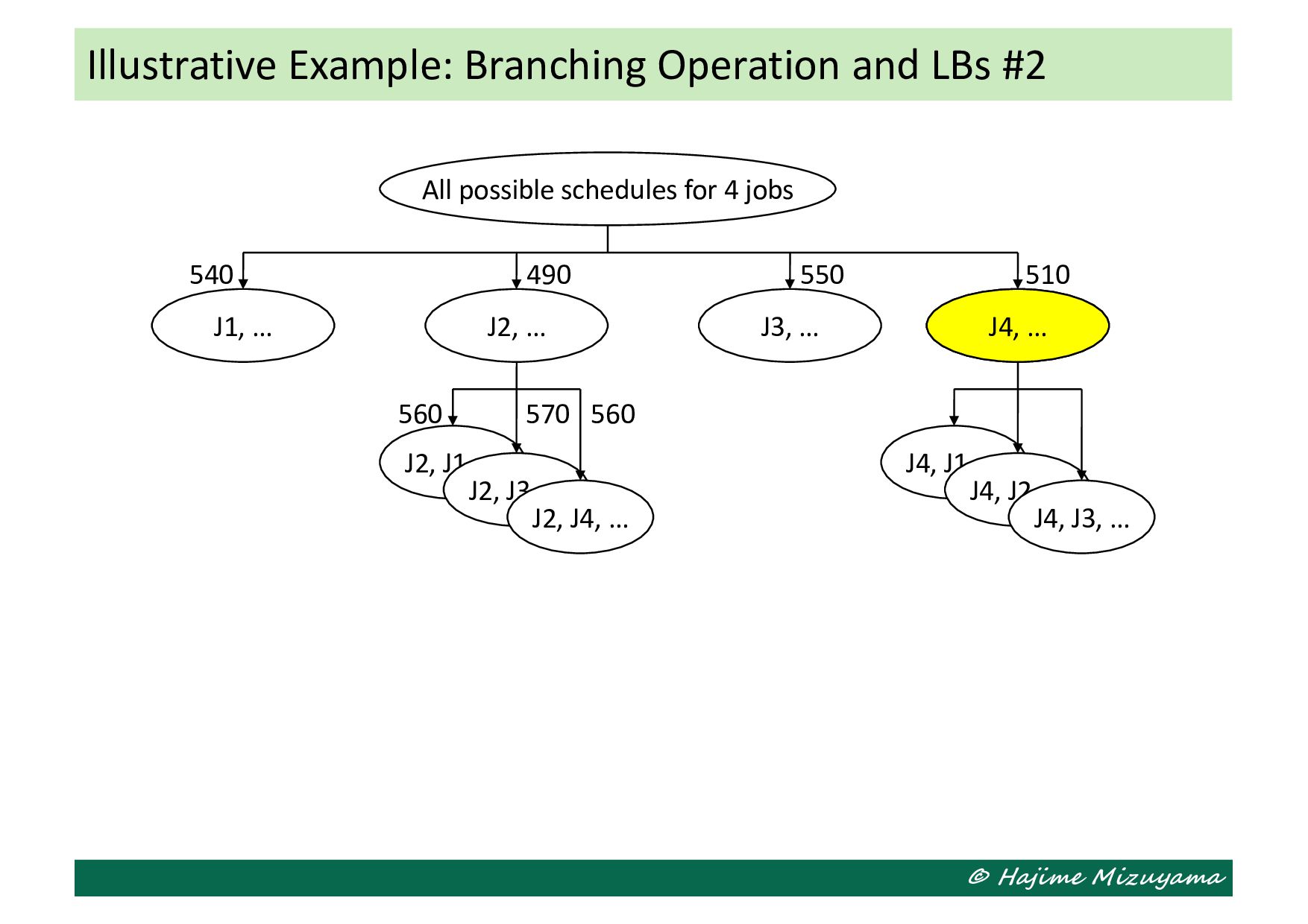
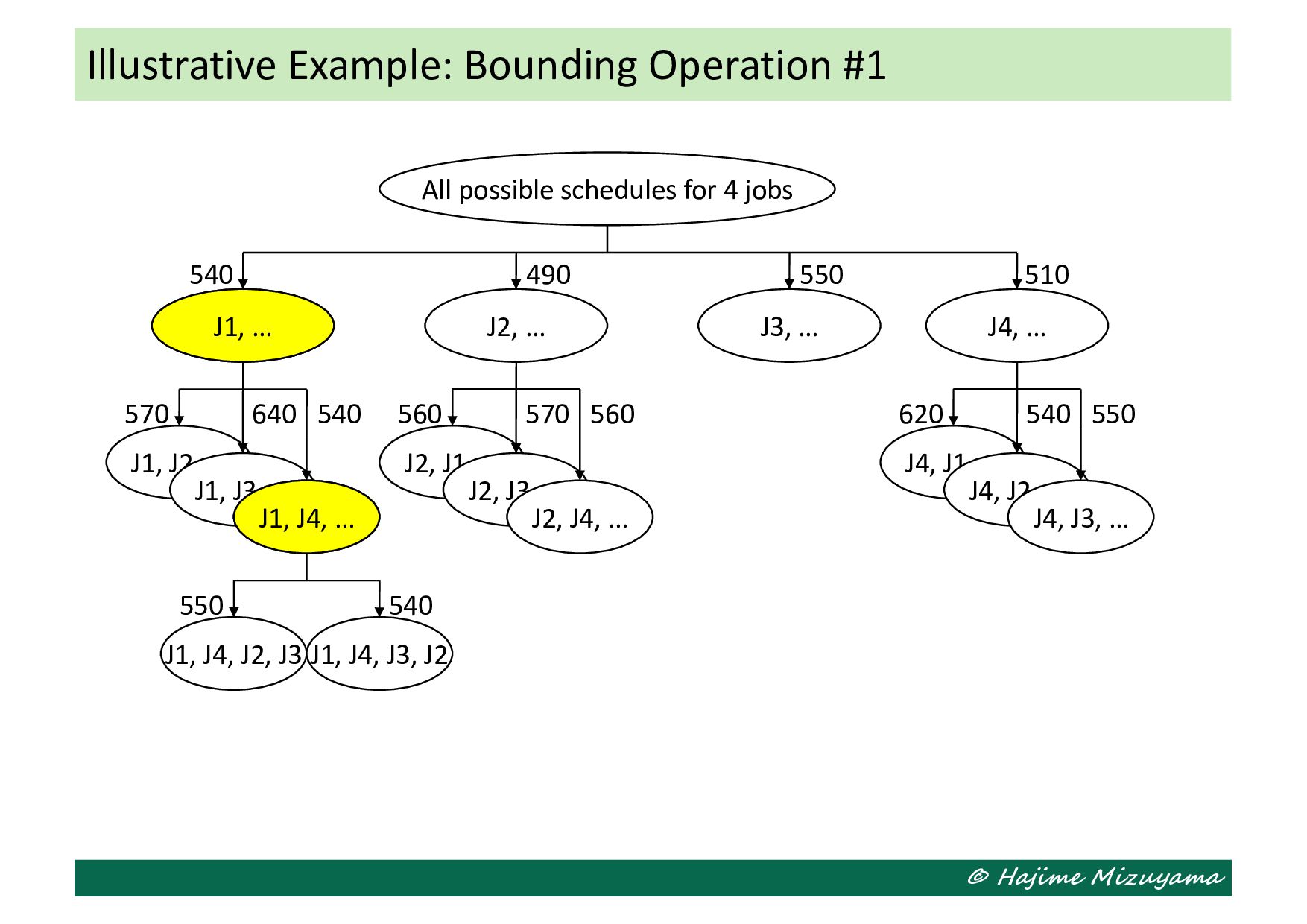
= {n0 }, where node n0 corresponds the set of all the feasible schedules (or job sequences). Step2: Take out a node from set N (and remove it from the set). Step3: Apply branching operation to the chosen node and calculate LB for each of its child nodes. Step4: For each child node, do the following: If it is a leaf node and LB < UB holds, replace (or define) the tentative solution with the schedule corresponding to the leaf node and apply bounding operation after setting UB = LB. If it is not a leaf node and LB < UB holds, add it to set N. Step5: Go back to Step2. Branch and Bound (BAB) Procedure
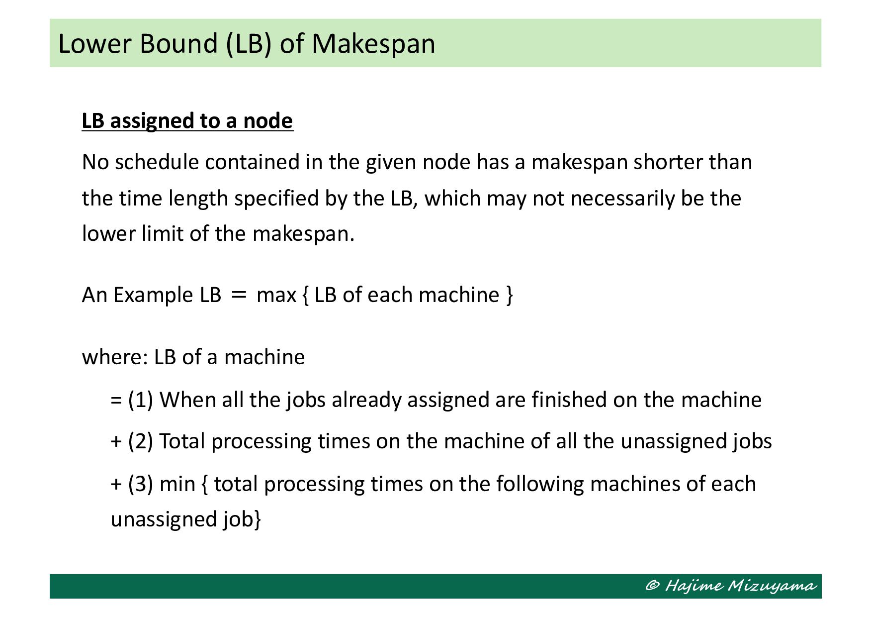
contained in the given node has a makespan shorter than the time length specified by the LB, which may not necessarily be the lower limit of the makespan. An Example LB = max { LB of each machine } where: LB of a machine = (1) When all the jobs already assigned are finished on the machine + (2) Total processing times on the machine of all the unassigned jobs + (3) min { total processing times on the following machines of each unassigned job} Lower Bound (LB) of Makespan
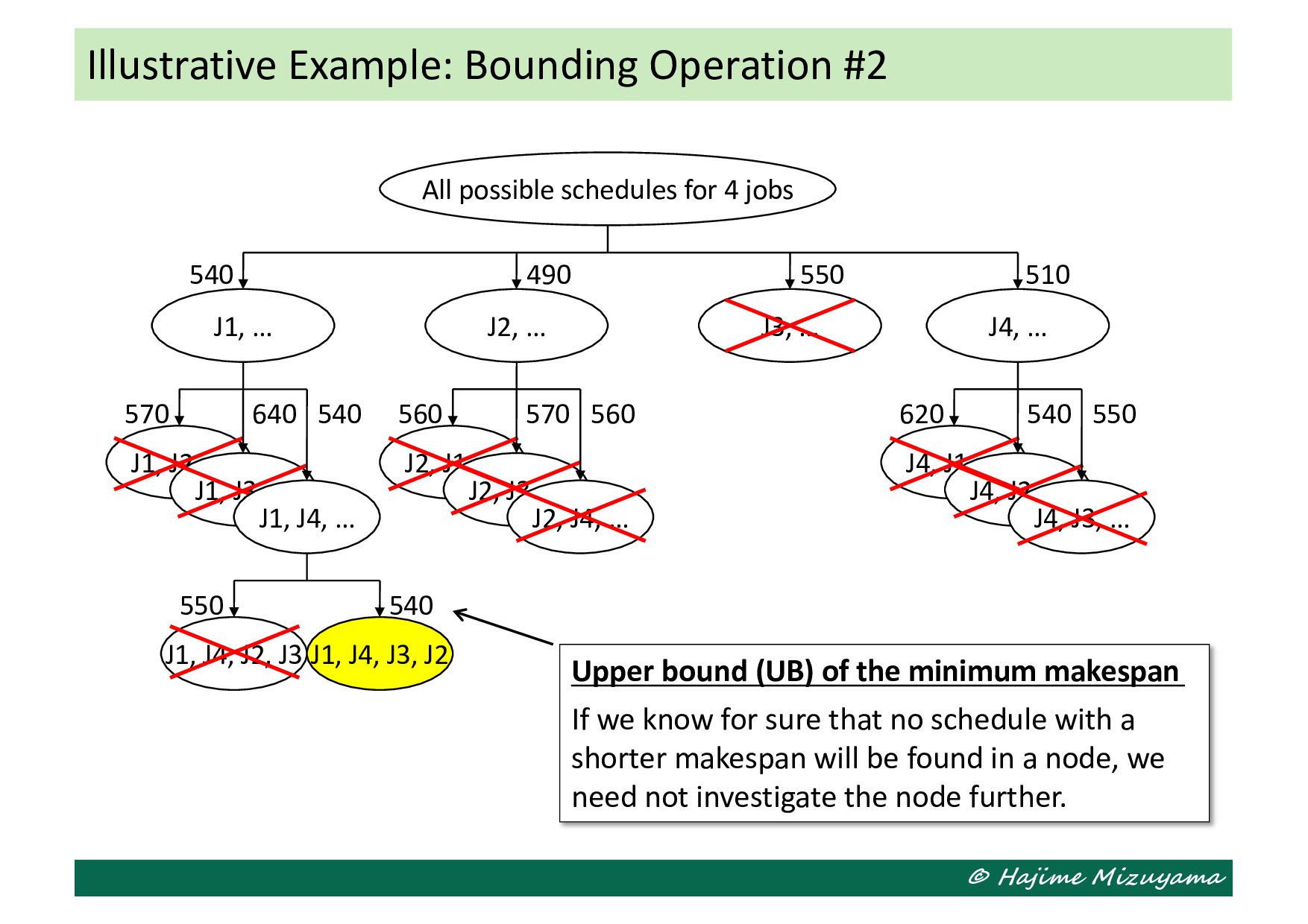
J1, … J2, J3, … J1, J2, … J1, J3, … Illustrative Example: Bounding Operation #2 All possible schedules for 4 jobs J2, … J1, … J4, … J3, … 540 490 550 510 J2, J4, … 560 570 560 J4, J3, … 620 540 550 J1, J4, … 570 640 540 J1, J4, J2, J3 J1, J4, J3, J2 550 540 Upper bound (UB) of the minimum makespan If we know for sure that no schedule with a shorter makespan will be found in a node, we need not investigate the node further.