Lecture slides for POM 2-11

生産管理技術2の講義11のスライドです．

Transcript

1. © Hajime Mizuyama Production & Operations Management #2 @AGU Lec.11: Scheduling Games and Mechanisms #1 • Game theoretical scheduling environment • Price of anarchy (POA) • Parallel machine scheduling examples
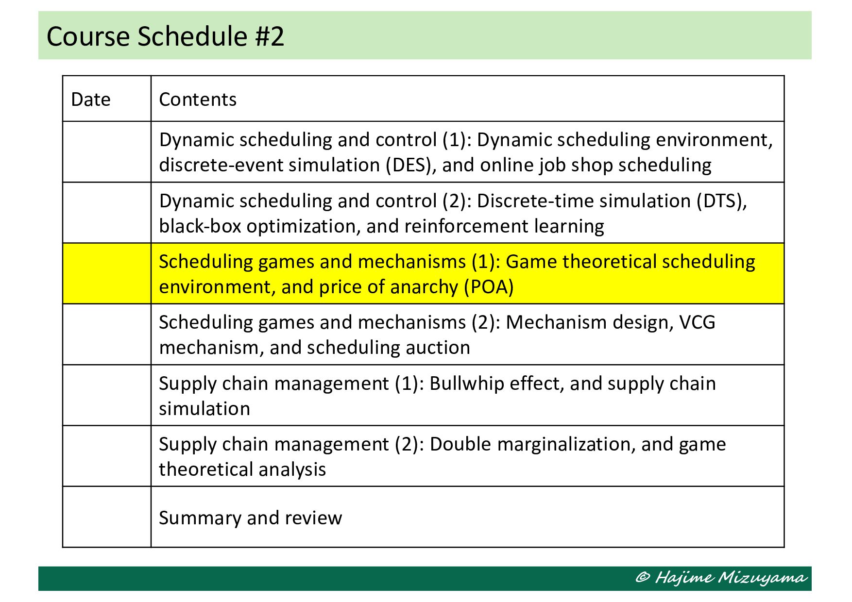
2. © Hajime Mizuyama Course Schedule #2 Date Contents Dynamic scheduling and control (1): Dynamic scheduling environment, discrete-event simulation (DES), and online job shop scheduling Dynamic scheduling and control (2): Discrete-time simulation (DTS), black-box optimization, and reinforcement learning Scheduling games and mechanisms (1): Game theoretical scheduling environment, and price of anarchy (POA) Scheduling games and mechanisms (2): Mechanism design, VCG mechanism, and scheduling auction Supply chain management (1): Bullwhip effect, and supply chain simulation Supply chain management (2): Double marginalization, and game theoretical analysis Summary and review
3. © Hajime Mizuyama • The owner of each job (or machine) may make a part of scheduling decision. For instance, job owners may have the option to select a machine from a given set of candidates for processing their job. • Some information necessary for making a schedule, such as, the weight, due date, tardiness penalty, etc. of each job, may be private information of its owner and unknown the the scheduler. • Similarly, the setup time, setup cost, available time slots, etc. of each machine may be private information of its owner and unknown the the scheduler. Game Theoretical Scheduling Environment
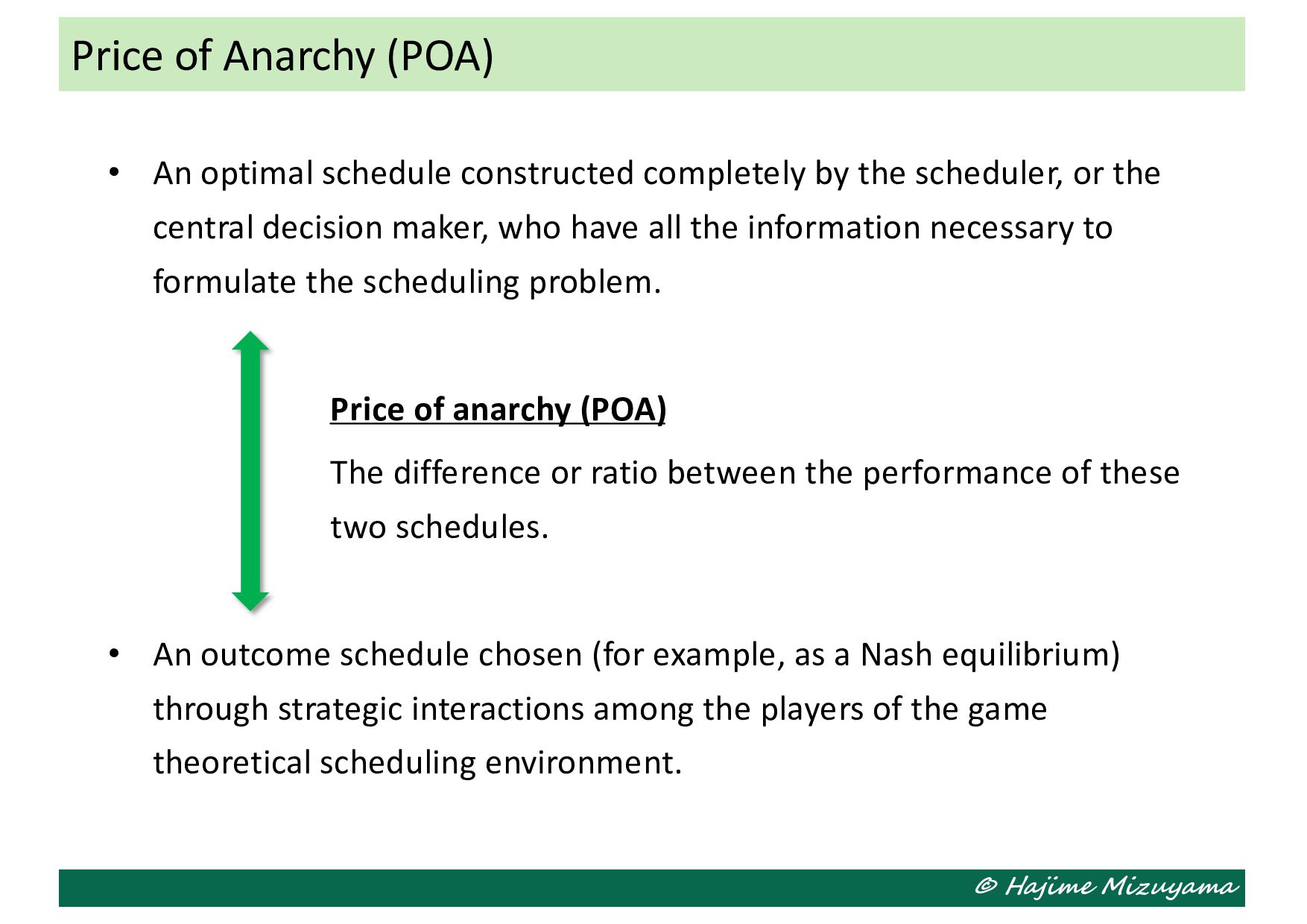
4. © Hajime Mizuyama • An optimal schedule constructed completely by the scheduler, or the central decision maker, who have all the information necessary to formulate the scheduling problem. Price of anarchy (POA) The difference or ratio between the performance of these two schedules. • An outcome schedule chosen (for example, as a Nash equilibrium) through strategic interactions among the players of the game theoretical scheduling environment. Price of Anarchy (POA)
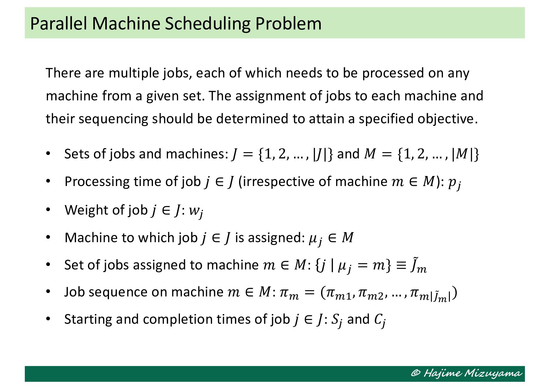
5. © Hajime Mizuyama There are multiple jobs, each of which needs to be processed on any machine from a given set. The assignment of jobs to each machine and their sequencing should be determined to attain a specified objective. • Sets of jobs and machines: 𝐽 = {1, 2, … , |𝐽|} and 𝑀 = {1, 2, … , |𝑀|} • Processing time of job 𝑗 ∈ 𝐽 (irrespective of machine 𝑚 ∈ 𝑀): 𝑝! • Weight of job 𝑗 ∈ 𝐽: 𝑤! • Machine to which job 𝑗 ∈ 𝐽 is assigned: 𝜇! ∈ 𝑀 • Set of jobs assigned to machine 𝑚 ∈ 𝑀: 𝑗 𝜇! = 𝑚} ≡ 2 𝐽" • Job sequence on machine 𝑚 ∈ 𝑀: 𝜋" = (𝜋"# , 𝜋"$ , … , 𝜋" % &! ) • Starting and completion times of job 𝑗 ∈ 𝐽: 𝑆! and 𝐶! Parallel Machine Scheduling Problem
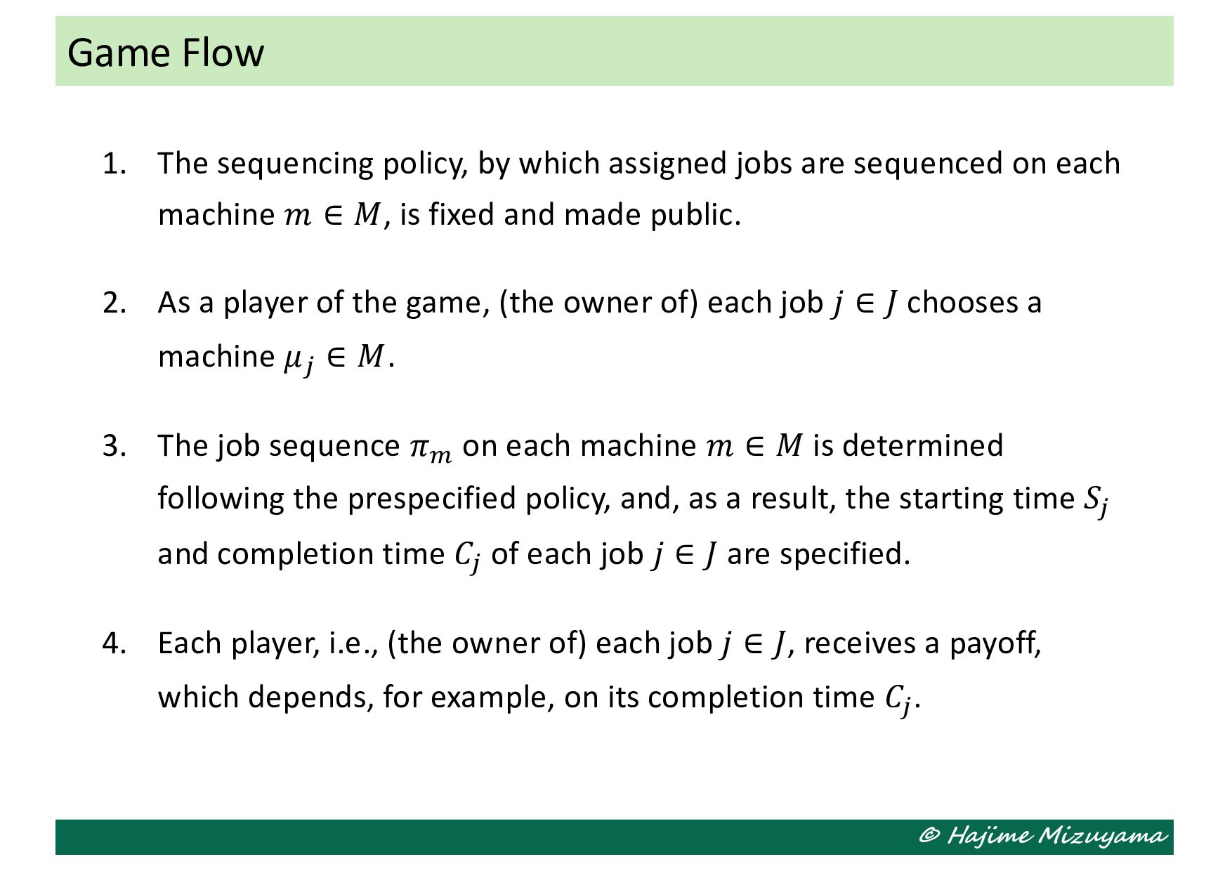
6. © Hajime Mizuyama 1. The sequencing policy, by which assigned jobs are sequenced on each machine 𝑚 ∈ 𝑀, is fixed and made public. 2. As a player of the game, (the owner of) each job 𝑗 ∈ 𝐽 chooses a machine 𝜇! ∈ 𝑀. 3. The job sequence 𝜋" on each machine 𝑚 ∈ 𝑀 is determined following the prespecified policy, and, as a result, the starting time 𝑆! and completion time 𝐶! of each job 𝑗 ∈ 𝐽 are specified. 4. Each player, i.e., (the owner of) each job 𝑗 ∈ 𝐽, receives a payoff, which depends, for example, on its completion time 𝐶!. Game Flow
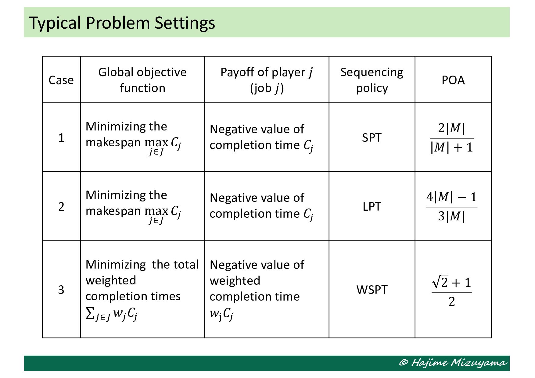
7. © Hajime Mizuyama Case Global objective function Payoff of player 𝑗 (job 𝑗) Sequencing policy POA 1 Minimizing the makespan max !∈# 𝐶! Negative value of completion time 𝐶! SPT 2|𝑀| 𝑀 + 1 2 Minimizing the makespan max !∈# 𝐶! Negative value of completion time 𝐶! LPT 4 𝑀 − 1 3|𝑀| 3 Minimizing the total weighted completion times ∑!∈# 𝑤! 𝐶! Negative value of weighted completion time 𝑤$ 𝐶! WSPT 2 + 1 2 Typical Problem Settings
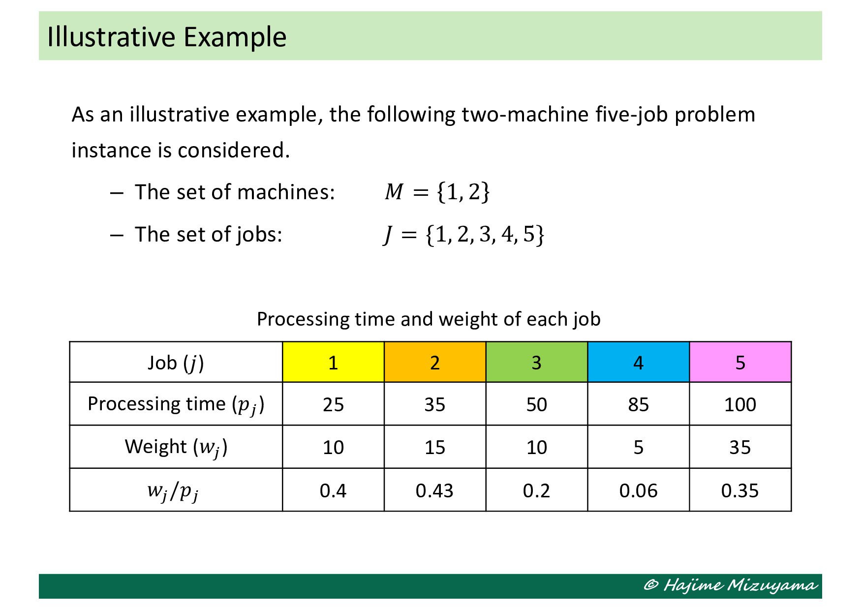
8. © Hajime Mizuyama As an illustrative example, the following two-machine five-job problem instance is considered. – The set of machines: 𝑀 = 1, 2 – The set of jobs: 𝐽 = {1, 2, 3, 4, 5} Illustrative Example Job (𝑗) 1 2 3 4 5 Processing time (𝑝! ) 25 35 50 85 100 Weight (𝑤! ) 10 15 10 5 35 𝑤! /𝑝! 0.4 0.43 0.2 0.06 0.35 Processing time and weight of each job
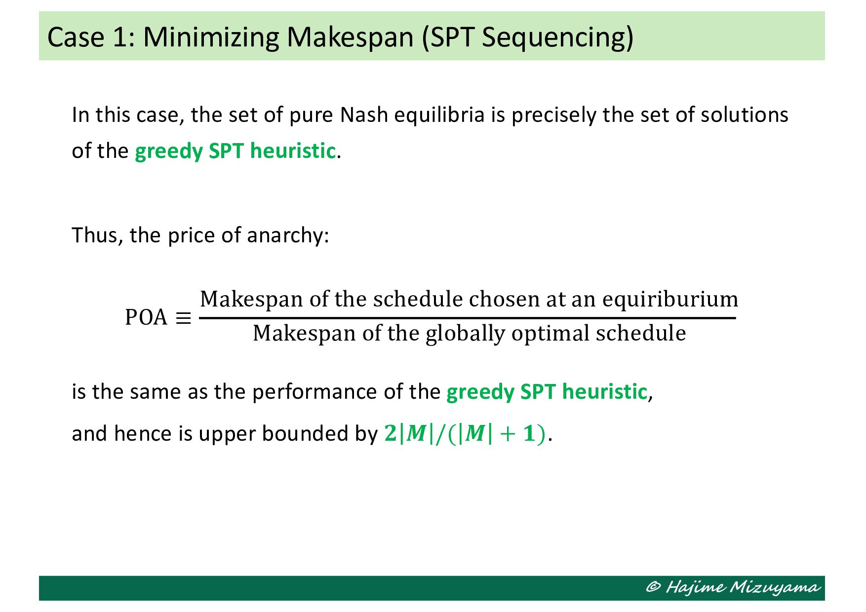
9. © Hajime Mizuyama In this case, the set of pure Nash equilibria is precisely the set of solutions of the greedy SPT heuristic. Thus, the price of anarchy: POA ≡ Makespan of the schedule chosen at an equiriburium Makespan of the globally optimal schedule is the same as the performance of the greedy SPT heuristic, and hence is upper bounded by 𝟐 𝑴 /( 𝑴 + 𝟏). Case 1: Minimizing Makespan (SPT Sequencing)
10. © Hajime Mizuyama 𝑁 ← 𝐽 𝐶" '() ← 0 (∀𝑚 ∈ 𝑀) while 𝑁 ≠ ∅ do 𝑗∗ ← argmin!∈, 𝑝! 𝑁 ← 𝑁 ∖ {𝑗∗} 𝜇!∗ ← argmin "∈- 𝐶" '() 𝐶.#∗ '() ← 𝐶.#∗ '() + 𝑝!∗ od Greedy SPT Heuristic
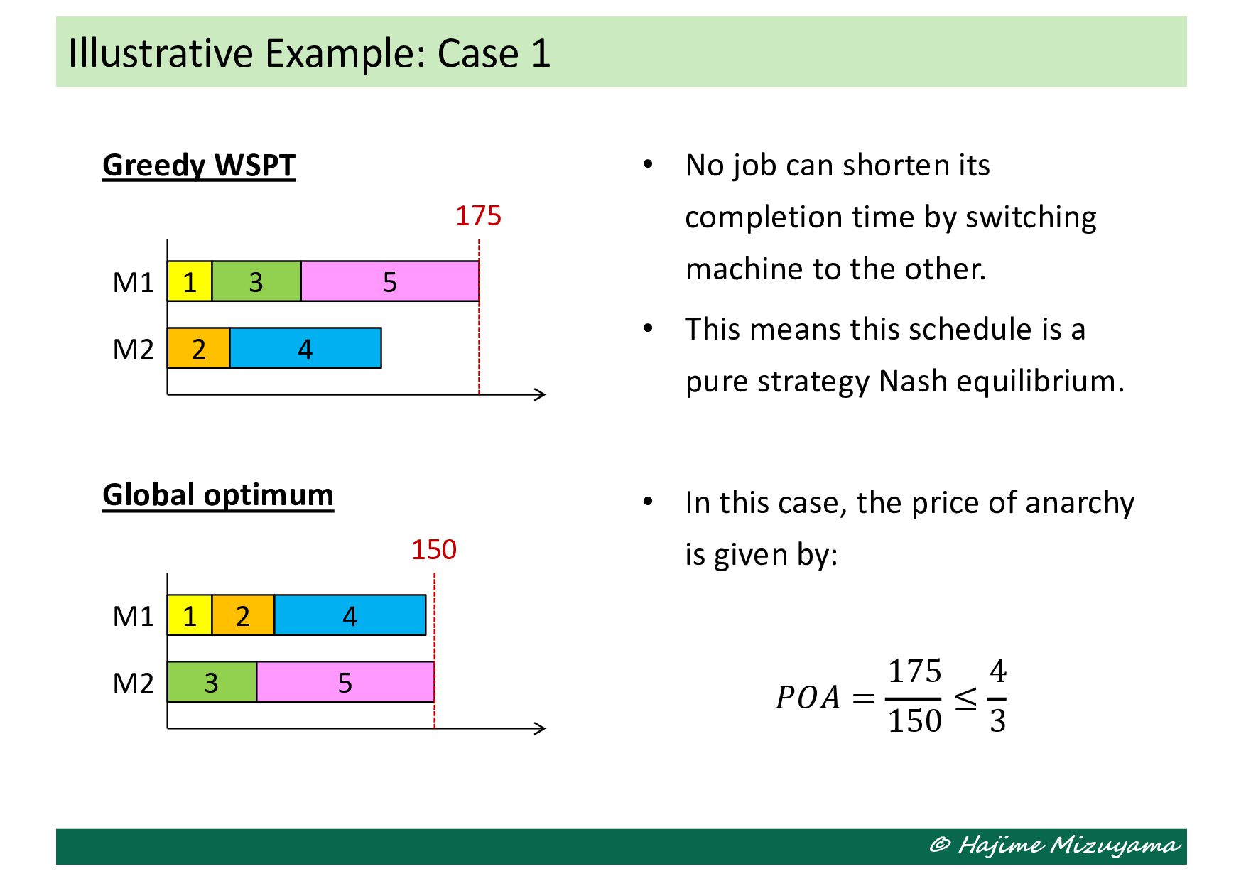
11. © Hajime Mizuyama Illustrative Example: Case 1 • No job can shorten its completion time by switching machine to the other. • This means this schedule is a pure strategy Nash equilibrium. • In this case, the price of anarchy is given by: 𝑃𝑂𝐴 = 175 150 ≤ 4 3 1 2 3 4 5 175 M1 M2 Greedy WSPT 1 2 3 4 5 150 M1 M2 Global optimum
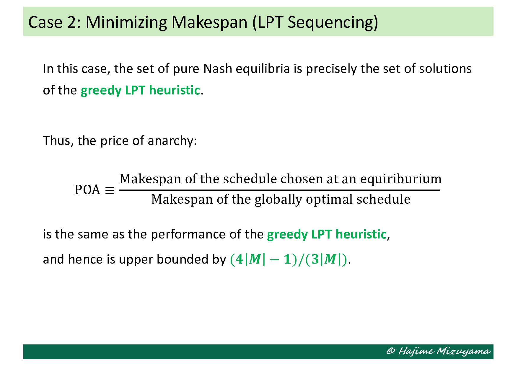
12. © Hajime Mizuyama In this case, the set of pure Nash equilibria is precisely the set of solutions of the greedy LPT heuristic. Thus, the price of anarchy: POA ≡ Makespan of the schedule chosen at an equiriburium Makespan of the globally optimal schedule is the same as the performance of the greedy LPT heuristic, and hence is upper bounded by (𝟒 𝑴 − 𝟏)/(𝟑 𝑴 ). Case 2: Minimizing Makespan (LPT Sequencing)
13. © Hajime Mizuyama 𝑁 ← 𝐽 𝐶" '() ← 0 (∀𝑚 ∈ 𝑀) while 𝑁 ≠ ∅ do 𝑗∗ ← argmax!∈, 𝑝! 𝑁 ← 𝑁 ∖ {𝑗∗} 𝜇!∗ ← argmin "∈- 𝐶" '() 𝐶.#∗ '() ← 𝐶.#∗ '() + 𝑝!∗ od Greedy LPT Heuristic
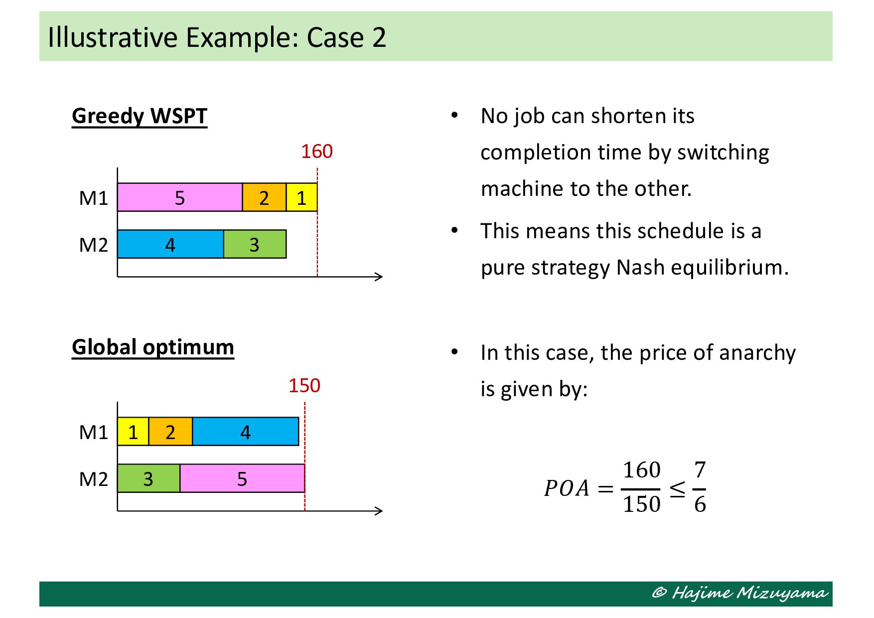
14. © Hajime Mizuyama Illustrative Example: Case 2 • No job can shorten its completion time by switching machine to the other. • This means this schedule is a pure strategy Nash equilibrium. • In this case, the price of anarchy is given by: 𝑃𝑂𝐴 = 160 150 ≤ 7 6 1 2 3 4 5 160 M1 M2 1 2 3 4 5 150 M1 M2 Greedy WSPT Global optimum
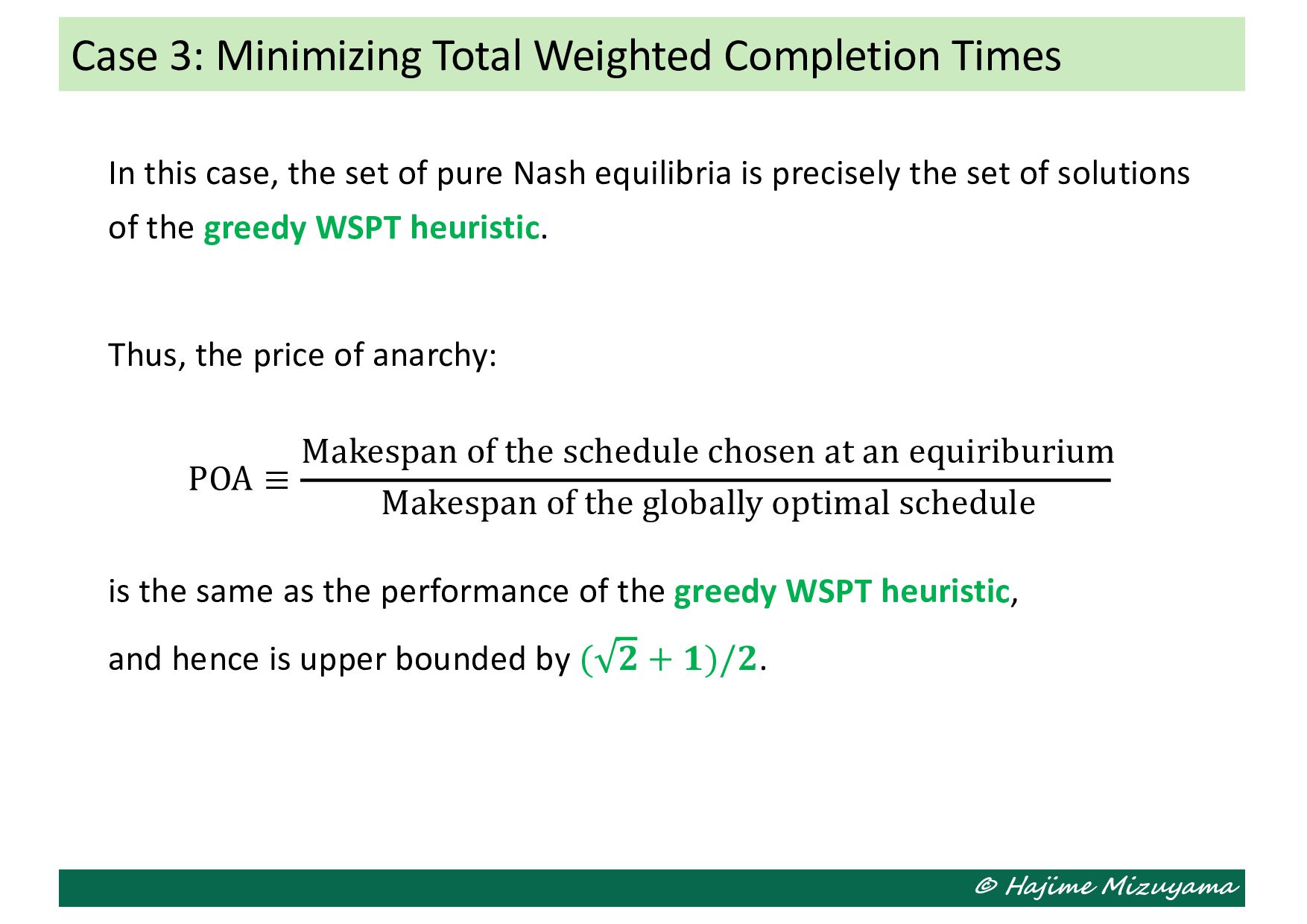
15. © Hajime Mizuyama In this case, the set of pure Nash equilibria is precisely the set of solutions of the greedy WSPT heuristic. Thus, the price of anarchy: POA ≡ Makespan of the schedule chosen at an equiriburium Makespan of the globally optimal schedule is the same as the performance of the greedy WSPT heuristic, and hence is upper bounded by ( 𝟐 + 𝟏)/𝟐. Case 3: Minimizing Total Weighted Completion Times
16. © Hajime Mizuyama 𝑁 ← 𝐽 𝐶" '() ← 0 (∀𝑚 ∈ 𝑀) while 𝑁 ≠ ∅ do 𝑗∗ ← argmax!∈, 𝑤! /𝑝! 𝑁 ← 𝑁 ∖ {𝑗∗} 𝜇!∗ ← argmin "∈- 𝐶" '() 𝐶.#∗ '() ← 𝐶.#∗ '() + 𝑝!∗ od Greedy WSPT Heuristic
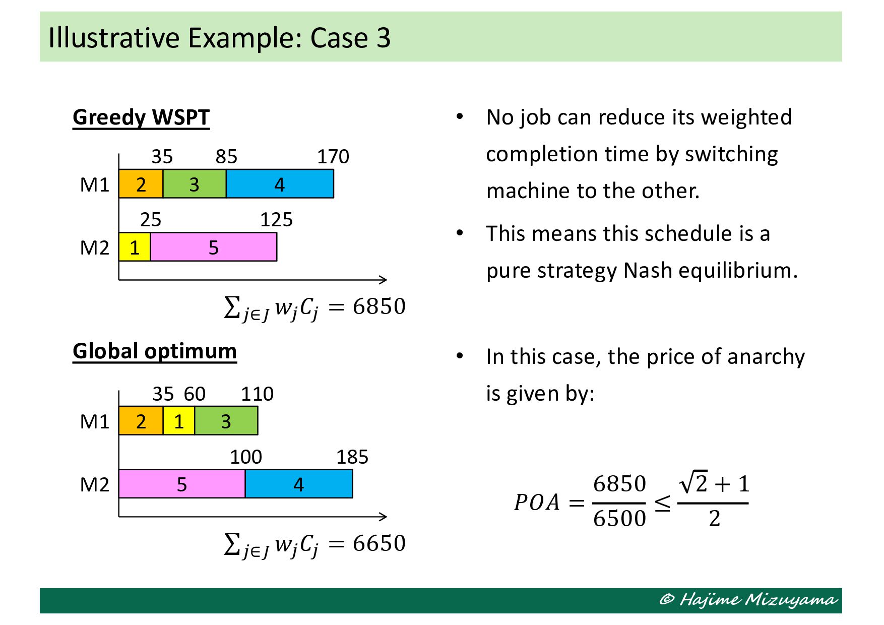
17. © Hajime Mizuyama Illustrative Example: Case 3 • No job can reduce its weighted completion time by switching machine to the other. • This means this schedule is a pure strategy Nash equilibrium. • In this case, the price of anarchy is given by: 𝑃𝑂𝐴 = 6850 6500 ≤ 2 + 1 2 1 2 3 4 5 M1 M2 Greedy WSPT 35 25 85 170 125 ∑!∈& 𝑤! 𝐶! = 6850 1 2 3 4 5 M1 M2 35 60 110 100 185 Global optimum ∑!∈& 𝑤! 𝐶! = 6650