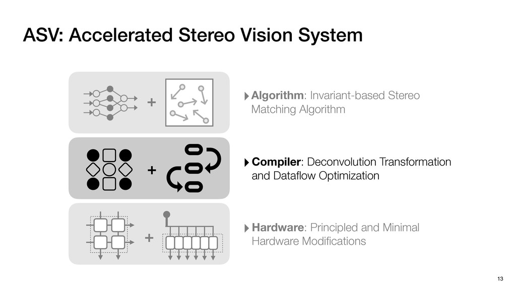
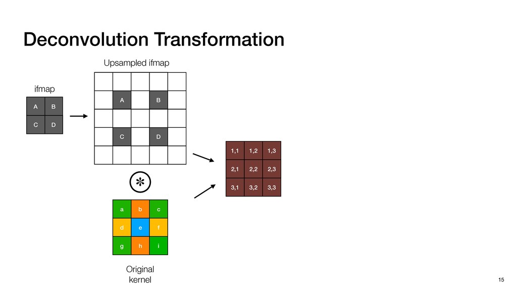
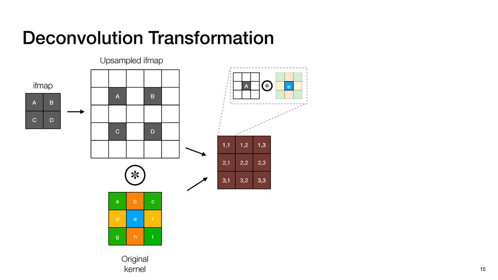
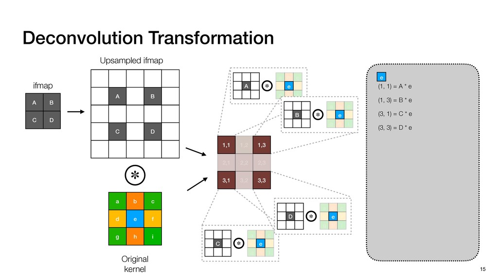
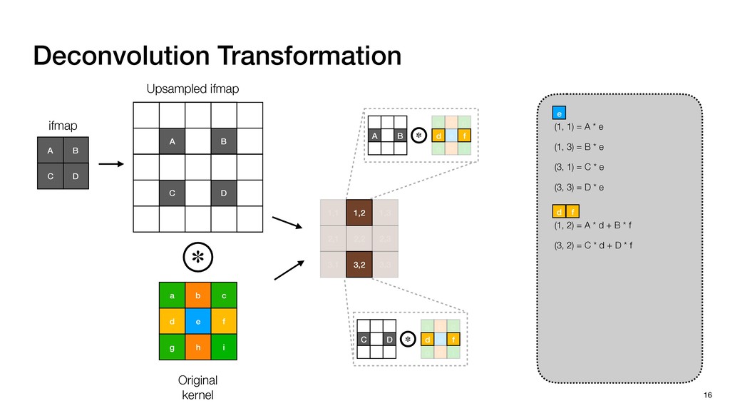
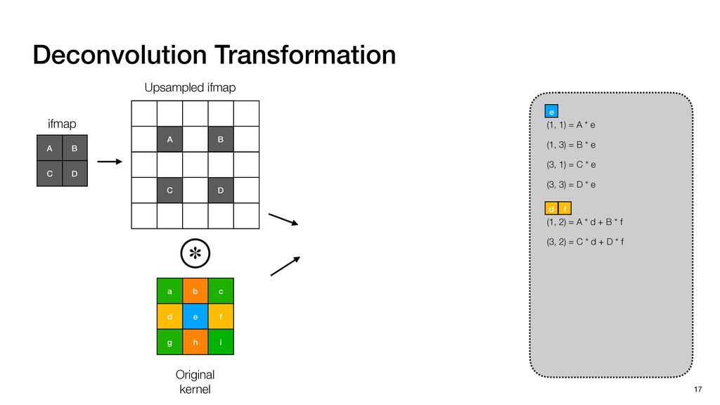
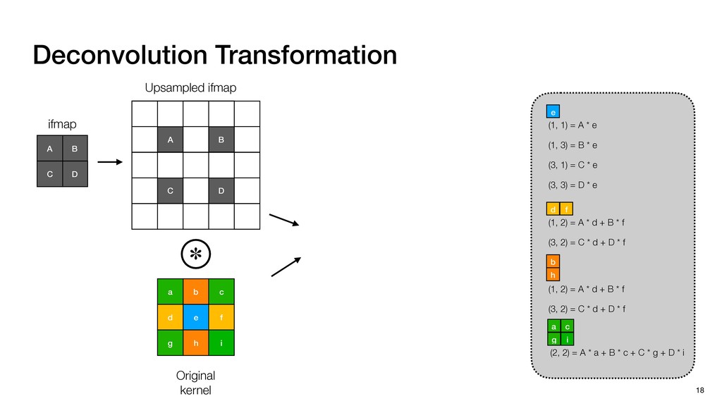
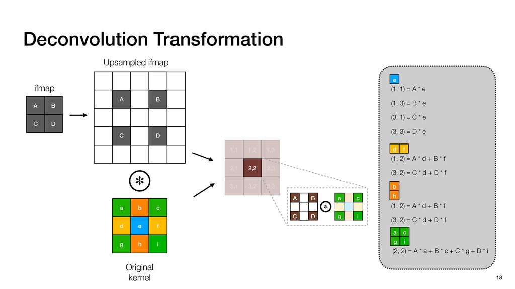
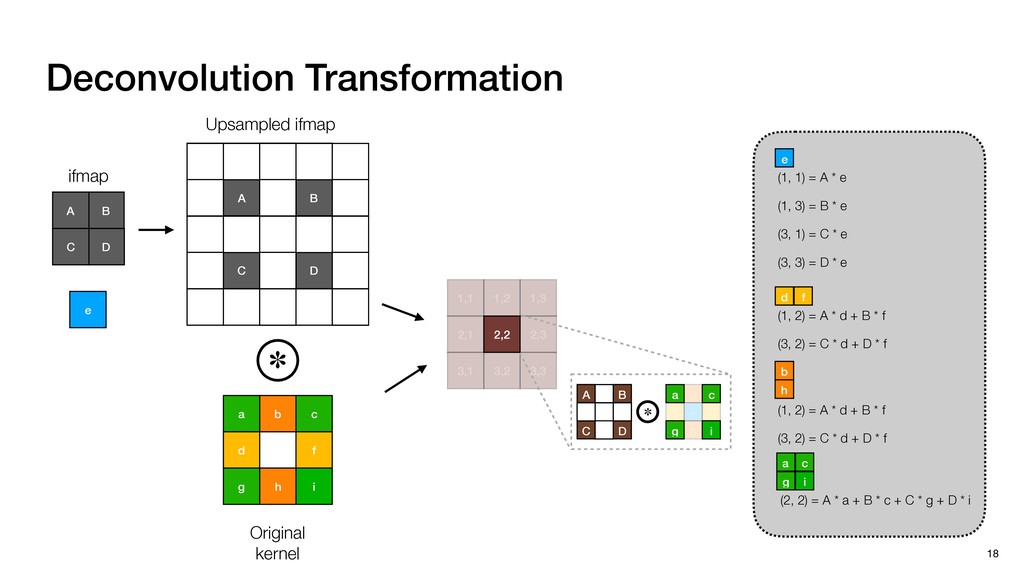
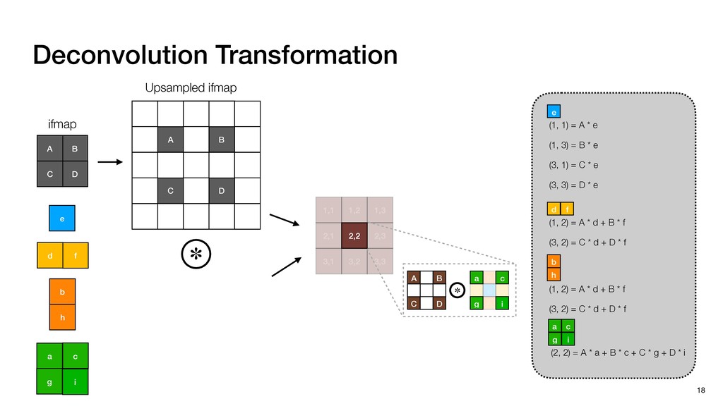
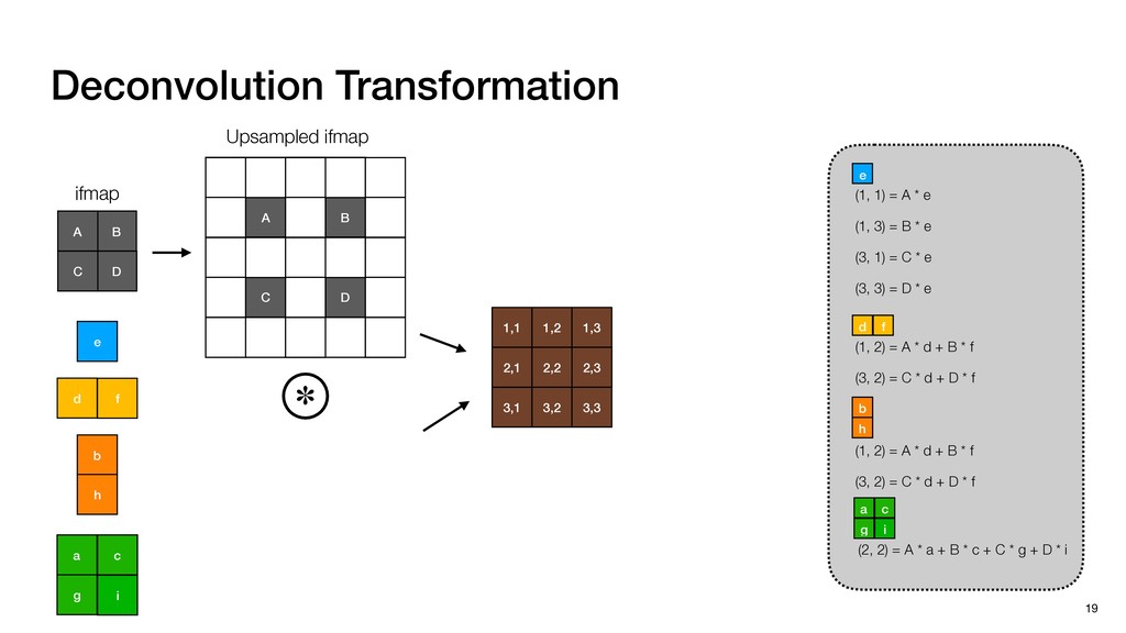
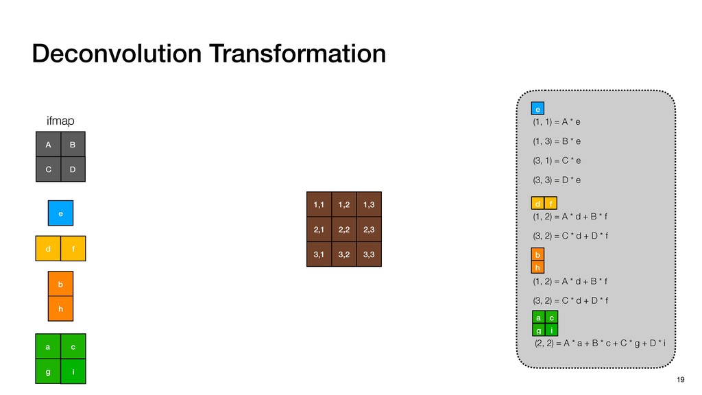
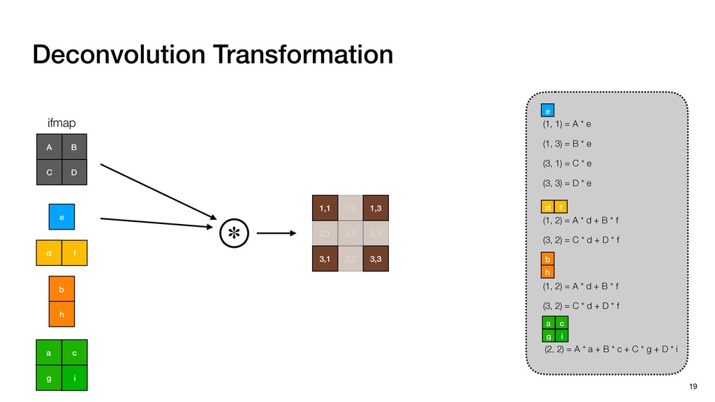
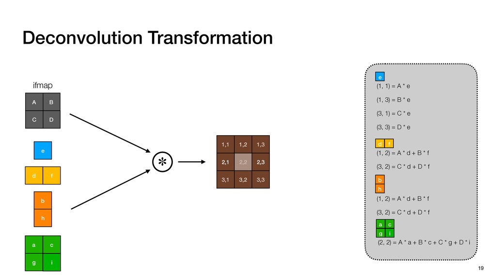
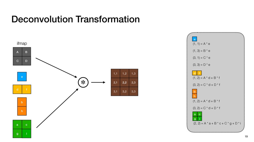
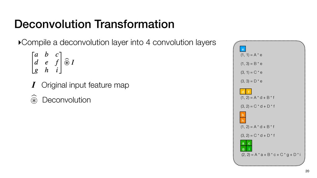
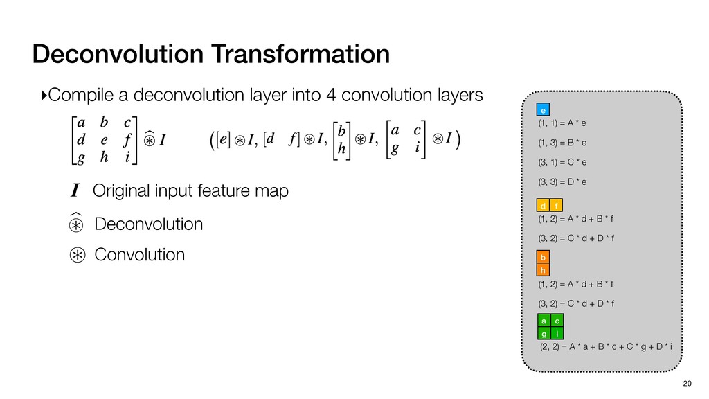
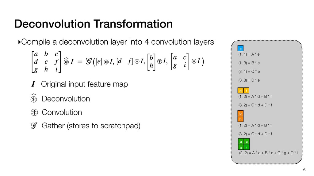
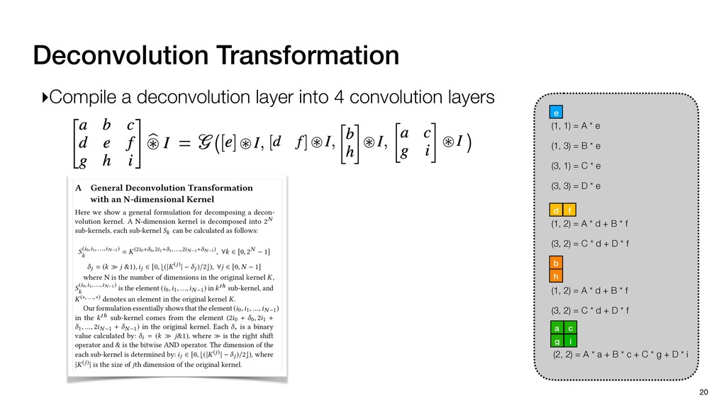
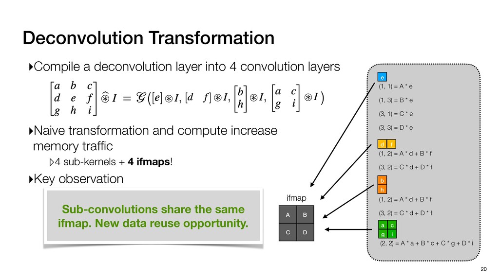
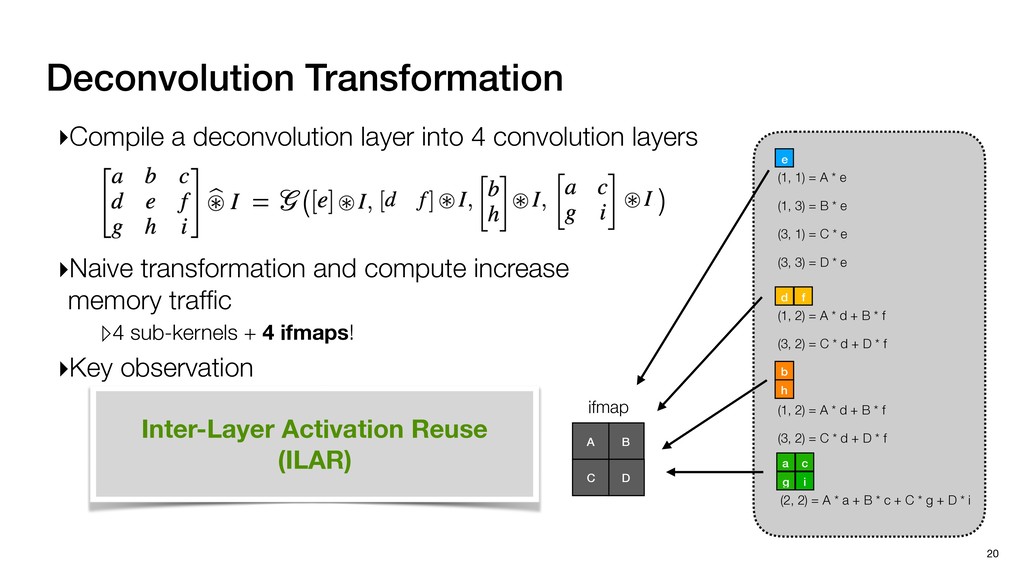
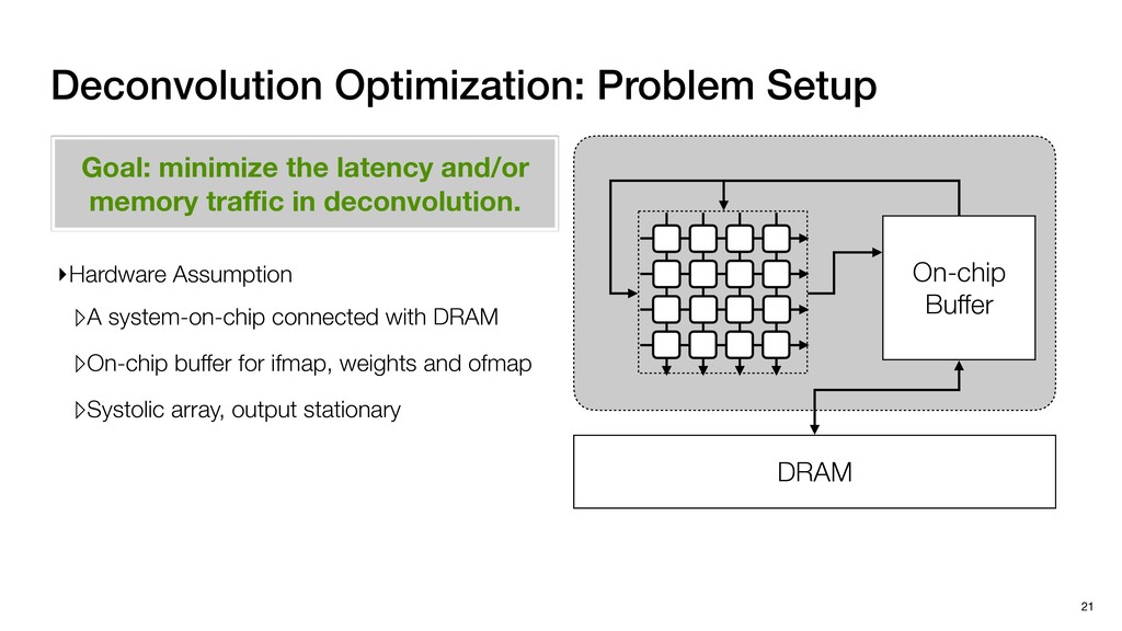
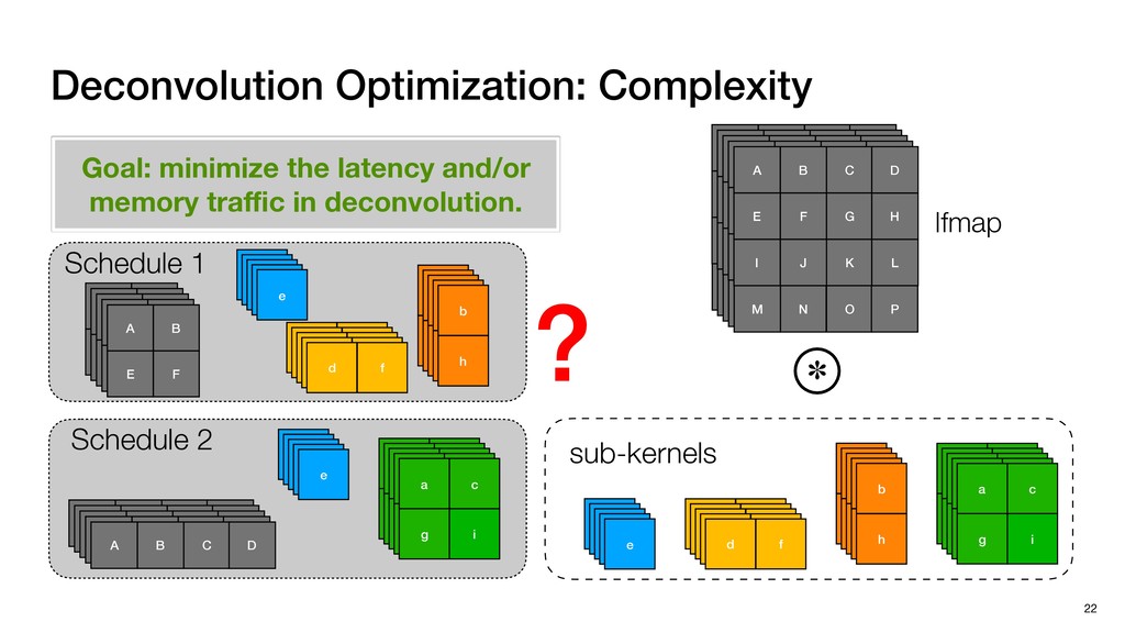
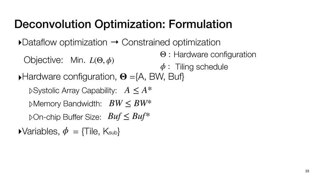
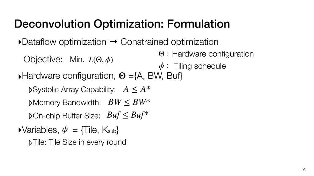
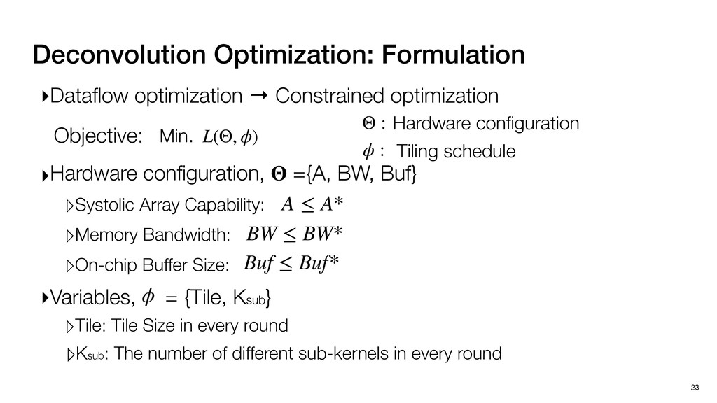
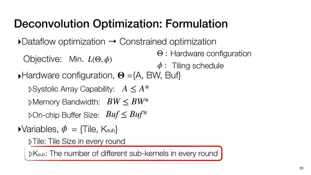
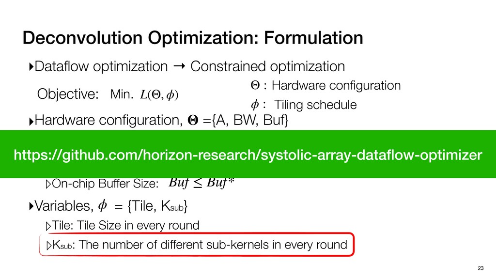
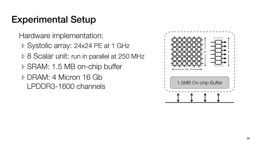
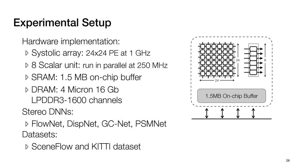
3) = B * e (3, 1) = C * e (3, 3) = D * e e (1, 2) = A * d + B * f (3, 2) = C * d + D * f f d (1, 2) = A * d + B * f (3, 2) = C * d + D * f b h ▸Compile a deconvolution layer into 4 convolution layers I Original input feature map e ofmap elements generated in this round are also stored he buffer, and are too shaded. terns. The key is to recognize that the four computation erns are essentially four different convolutions, each con- ving the original ifmap with a distinct kernel that is part he original kernel. For instance, (2, 2), (2, 4), (4, 2), and 4) are generated by convolving ⇥ a c g i ⇤ with ifmap. More erally, the deconvolution in Fig. 6 can be calculated as: b c e f h i # b ~ I = G ([e]~I,[d f]~I, b h ~I, a c g i ~I) ere b ~ denotes deconvolution, ~ denotes standard convolu- n, I denotes the ifmap, and G denotes the gather operation t assembles the ofmap from the results of the four con- utions. G can be simply implemented as a set of load rations to the scratchpad memory (on-chip buffer). Essentially, our algorithm decomposes the original 3⇥3 cient for convolutions. also be extended to supp which have more relaxe We assume that the ac (scratchpad memory) th as output elements. The hold all the data for a lay in multiple rounds. Onl loaded into the buffer ea into the buffer in each ro and is determined by th The buffer is evenly s buffer to support doub computing the current ro data needed for the next The next round does no This design choice guara Deconvolution ents generated in this round are also stored d are too shaded. y is to recognize that the four computation ntially four different convolutions, each con- nal ifmap with a distinct kernel that is part ernel. For instance, (2, 2), (2, 4), (4, 2), and ted by convolving ⇥ a c g i ⇤ with ifmap. More convolution in Fig. 6 can be calculated as: = G ([e]~I,[d f]~I, b h ~I, a c g i ~I) deconvolution, ~ denotes standard convolu- e ifmap, and G denotes the gather operation he ofmap from the results of the four con- n be simply implemented as a set of load cient for convolutions. Alte also be extended to support which have more relaxed co We assume that the accele (scratchpad memory) that h as output elements. The bu hold all the data for a layer. T in multiple rounds. Only pa loaded into the buffer each r into the buffer in each round and is determined by the lo The buffer is evenly split buffer to support double-b computing the current round data needed for the next rou Convolution h a 3⇥3 kernel split into four sub-kernels. With a tiling strategy W = 2,H = 2,C1 = 1,C2 = 2,C3 = only the shaded elements are loaded into the buffer. p elements generated in this round are also stored fer, and are too shaded. The key is to recognize that the four computation re essentially four different convolutions, each con- he original ifmap with a distinct kernel that is part ginal kernel. For instance, (2, 2), (2, 4), (4, 2), and generated by convolving ⇥ a c g i ⇤ with ifmap. More , the deconvolution in Fig. 6 can be calculated as: c f i # b ~ I = G ([e]~I,[d f]~I, b h ~I, a c g i ~I) denotes deconvolution, ~ denotes standard convolu- notes the ifmap, and G denotes the gather operation mbles the ofmap from the results of the four con- sists of a 2D systolic array, in whic (PE) performs one MAC operation arrays use a simple neighbor-to- mechanism that simplifies the con cient for convolutions. Alternativ also be extended to support SIMD- which have more relaxed control w We assume that the accelerator h (scratchpad memory) that holds ac as output elements. The buffer siz hold all the data for a layer. Therefo in multiple rounds. Only part of th loaded into the buffer each round. E into the buffer in each round is criti and is determined by the loop tilin The buffer is evenly split into a w buffer to support double-bufferin computing the current round using data needed for the next round is p Gather (stores to scratchpad) c a i g (2, 2) = A * a + B * c + C * g + D * i ( ) =