VS in FDA Short Course II

Transcript

1. 1 SHORT COURSE: VARIABLE SELECTION IN SCALAR-ON-FUNCTION MODELS JEFF GOLDSMITH, PHD DEPARTMENT OF BIOSTATISTICS
2. 2 Linear SoFR with one predictor yi = 0 + Z xi( t ) ( t ) dt + ✏i • Scalar response yi • Functional predictor xi (t) • Functional covariate is of interest • Linear model • Most common approach
3. 3 Basis expansion • The functional coefficient is usually expanded in terms of a basis; the predictor sometimes is as well • Several basis options are possible • FPC • Splines (my preference) • Wavelets • Fourier
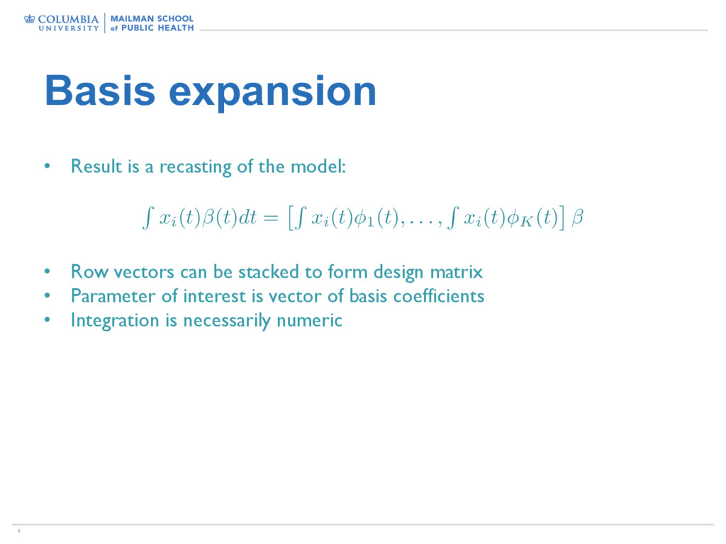
4. 4 Basis expansion • Result is a recasting of the model: R xi( t ) ( t ) dt = ⇥R xi( t ) 1( t ) , . . . , R xi( t ) K( t ) ⇤ • Row vectors can be stacked to form design matrix • Parameter of interest is vector of basis coefficients • Integration is necessarily numeric
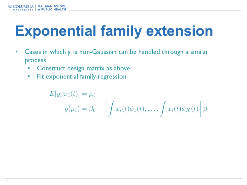
5. 5 Exponential family extension • Cases in which yi is non-Gaussian can be handled through a similar process • Construct design matrix as above • Fit exponential family regression E [ yi | xi( t )] = µi g ( µi) = 0 + Z xi( t ) 1( t ) , . . . , Z xi( t ) K( t )
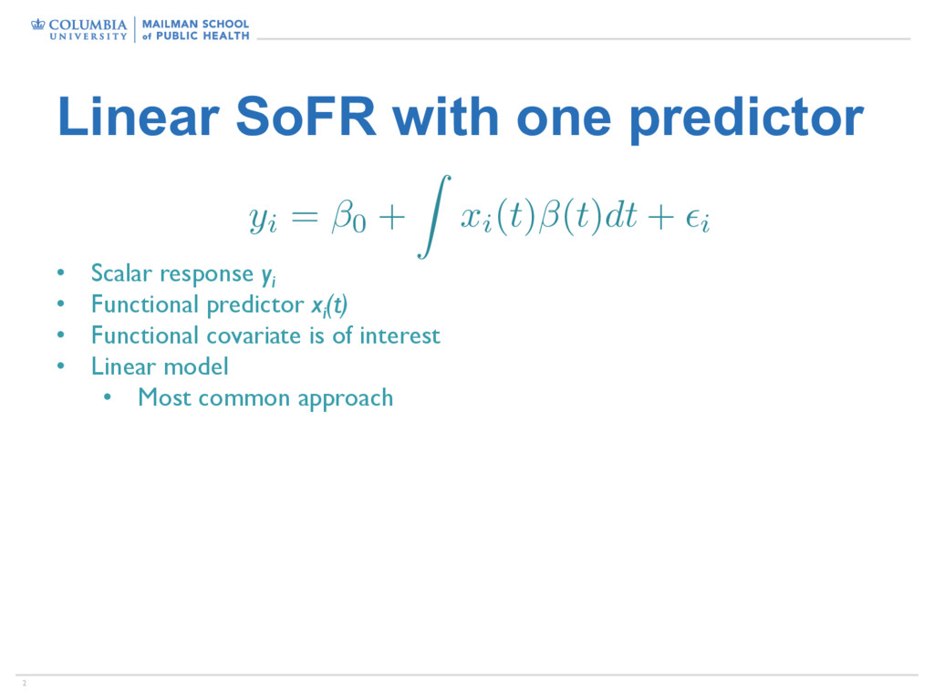
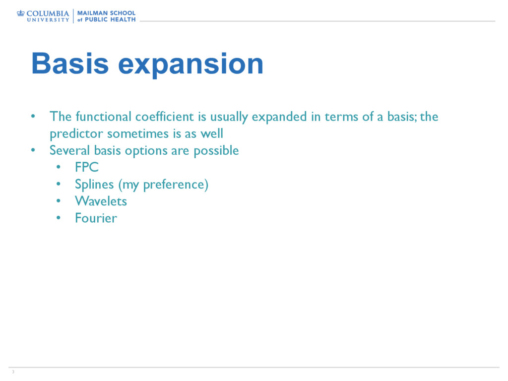
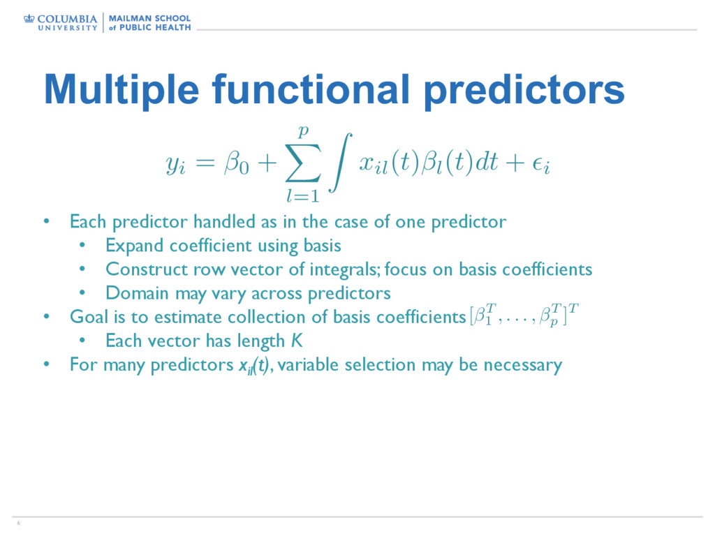
6. 6 Multiple functional predictors • Each predictor handled as in the case of one predictor • Expand coefficient using basis • Construct row vector of integrals; focus on basis coefficients • Domain may vary across predictors • Goal is to estimate collection of basis coefficients • Each vector has length K • For many predictors xil (t), variable selection may be necessary yi = 0 + p X l=1 Z xil( t ) l( t ) dt + ✏i [ T 1 , . . . , T p ]T
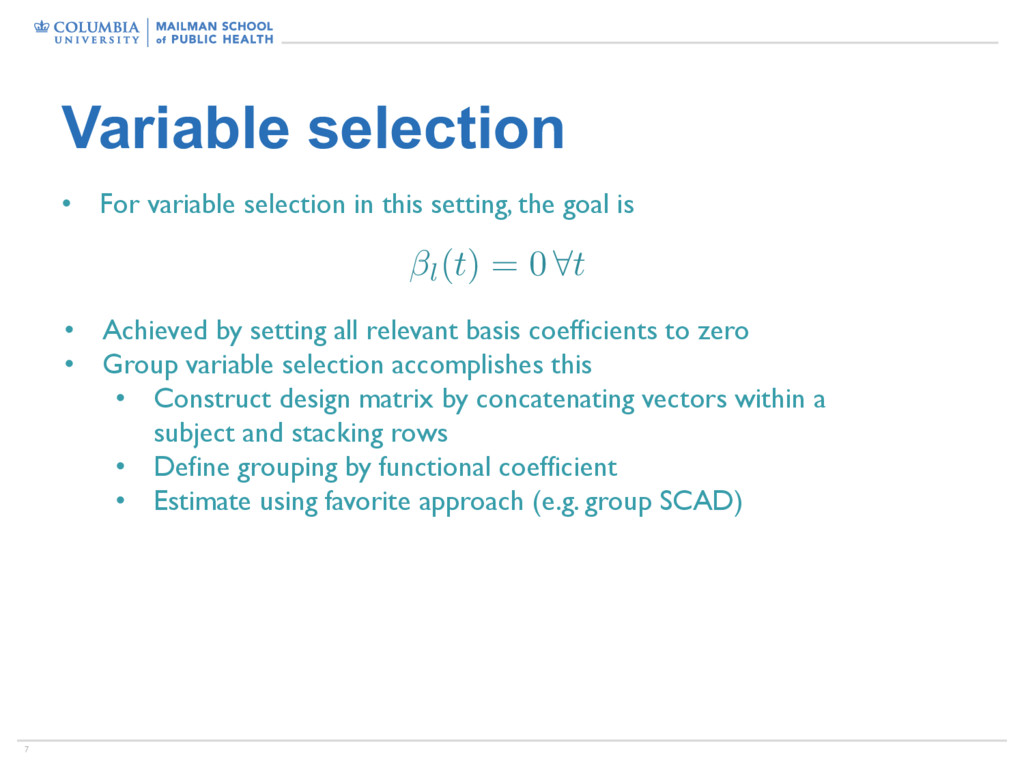
7. 7 Variable selection • For variable selection in this setting, the goal is l(t) = 0 8t • Achieved by setting all relevant basis coefficients to zero • Group variable selection accomplishes this • Construct design matrix by concatenating vectors within a subject and stacking rows • Define grouping by functional coefficient • Estimate using favorite approach (e.g. group SCAD)
8. 8 Scaling predictors • In variable selection settings, common to scale predictors to have mean 0 and variance 1 • Ensures that coefficients for predictors with high variability aren’t over penalized • In this setting, can be done pointwise over t
9. 9 Sparse or incomplete data • Not always necessary to smooth the predictors, but in the case of noisy, sparse, or incomplete predictors this may be necessary • Not a problem to do routinely, either • In this case, the integration is between the smoothed predictor evaluated over a reasonable domain
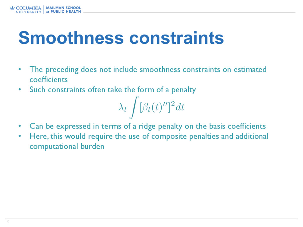
10. 10 Smoothness constraints • The preceding does not include smoothness constraints on estimated coefficients • Such constraints often take the form of a penalty l Z [ l(t)00]2dt • Can be expressed in terms of a ridge penalty on the basis coefficients • Here, this would require the use of composite penalties and additional computational burden
11. 11 Key references • Ramsay and Silverman (2005). Functional data analysis. • Gertheiss et al (2013). Variable Selection in Generalized Functional Linear Models. Stat.
12. 12 Switch to code