psb_fridley

Transcript

1. Workshop #1: Statistical analysis of single-cell protein data Pacific Symposium of Biocomputing (PSB) January 2024
2. Speakers • Brooke L Fridley, PhD Moffitt Cancer Center Children’s Mercy Hospital • Simon Vandekar Vanderbilt University Medical Center • Inna Chervoneva Thomas Jefferson University • Julia Wrobel Emory University • Siyuan Ma Vanderbilt University Medical Center
3. Schedule 9:00 –9:10: Welcome and Introduction of workshop and speakers. 9:10 – 9:40: Speaker 1: Brooke Fridley Title: Overview of abundance-based and spatial-based analysis approaches for multiplex imaging data 9:40 – 9:45: Questions for speaker 1 9:45 – 10:10: Speaker 2: Simon Vandekar Title: Normalization and Cell Phenotyping for mIF data 10:10 – 10:15: Questions for speaker 2 10:15– 10:40: Speaker 3: Inna Chervoneva Title: Quantile biomarkers based on single-cell multiplex immunofluorescence imaging data 10:40 – 10:45: Questions for speaker 3 10:45 – 11:10: Speaker 4: Julia Wrobel Title: Tools and software for functional data analysis of multiplexed imaging data 11:10 – 11:15: Questions for speaker 4 11:15 – 11:40: Speaker 5: Siyuan Ma Title: A Flexible Generalized Linear Mixed Effects Model for Testing Cell-Cell Colocalization in Spatial Immunofluorescent Data 11:40 – 11:45: Questions for speaker 5 11:45 – Noon: Panel discussion and questions 3
4. Overview of abundance-based and spatial-based analysis approaches for multiplex imaging data Brooke L. Fridley, PhD Professor Director, Biostatistics & Epidemiology Core Children’s Mercy Hospital Kansas City, MO
5. TIME and Multiplex immunofluorescence (mIF) • The recent development of immunotherapies has ushered in a new era of cancer treatment. • These therapeutics have led to revolutionary breakthroughs; however, the efficacy has been modest and is often restricted to a subset of patients. • Hence, identification of which cancer patients will benefit from immunotherapy is essential. • Multiplex immunofluorescence (mIF) microscopy allows for the assessment and visualization of the tumor microenvironment (TME). 5
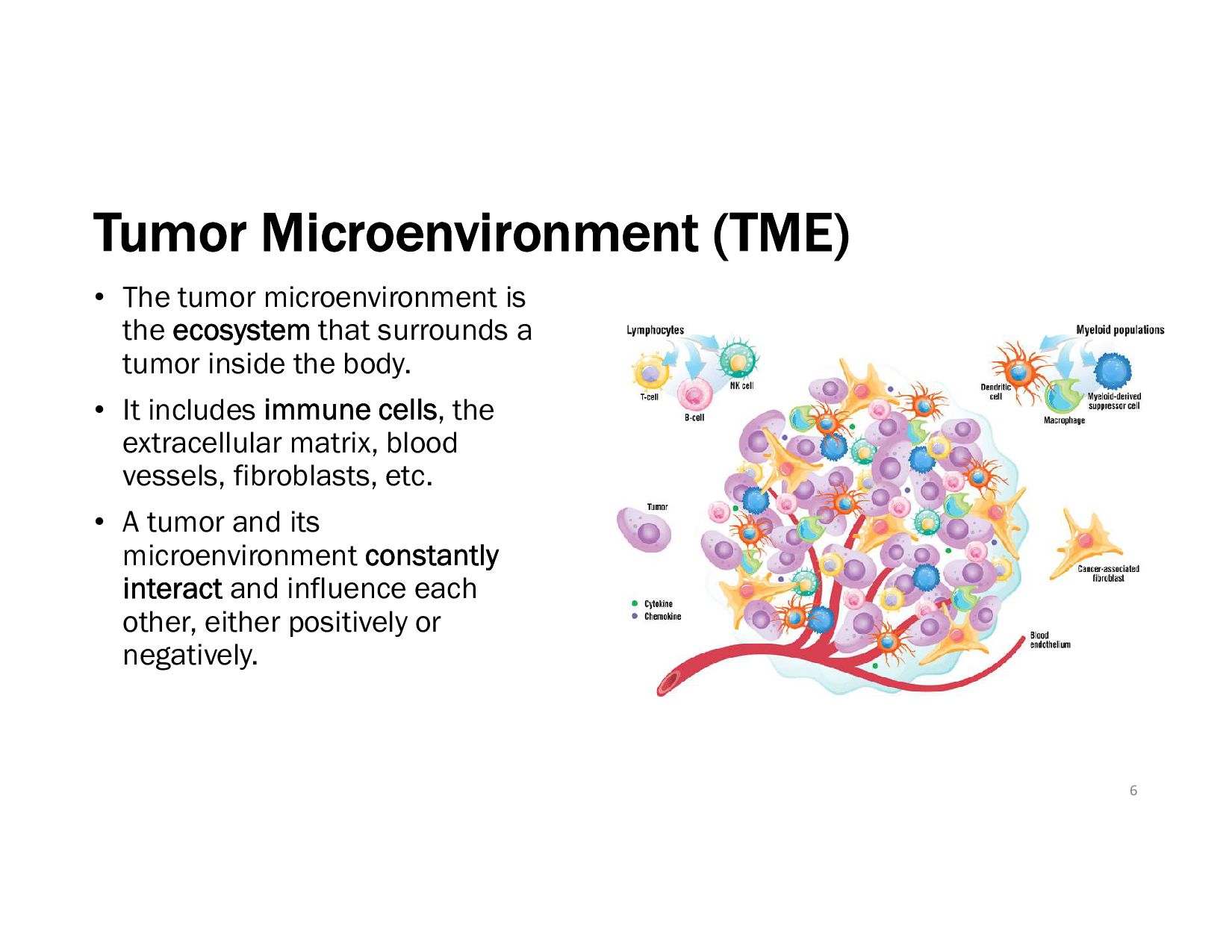
6. Tumor Microenvironment (TME) • The tumor microenvironment is the ecosystem that surrounds a tumor inside the body. • It includes immune cells, the extracellular matrix, blood vessels, fibroblasts, etc. • A tumor and its microenvironment constantly interact and influence each other, either positively or negatively. 6
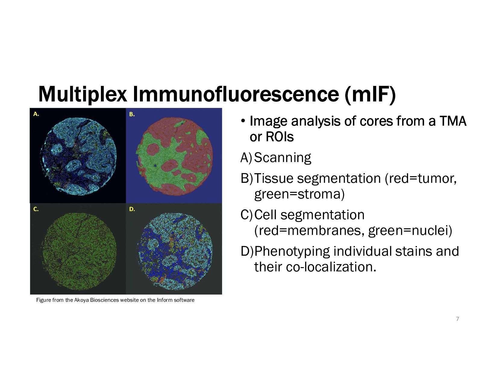
7. Multiplex Immunofluorescence (mIF) • Image analysis of cores from a TMA or ROIs A)Scanning B)Tissue segmentation (red=tumor, green=stroma) C)Cell segmentation (red=membranes, green=nuclei) D)Phenotyping individual stains and their co-localization. 7 Figure from the Akoya Biosciences website on the Inform software
8. Cell types represented by Markers • Also have markers for various function, such as activation (CD69) and exhaustion (TIM3, LAG3)
9. AACES Ovarian Cancer Study of TME with mIF • African American with HGSC EOC • 94 subject with 263 TMA cores • 93 subjects with 260 on ROIs (intra-tumoral) • 27 subjects on both TMA and ROIs • Vectra 3.0 (Akoya Biosciences) with images are exported from InForm (Akoya Biosciences) and loaded into HALO (Indica Labs) for quantitative image analysis • Markers: 1. Pancytokeratin/PCK = tissue segmentation 2. DAPI = cell segmentation 3. CD3+ = tumor infiltrating lymphocytes 4. CD3+CD8+ = cytotoxic T-cells 5. CD3+FoxP3+ = regulatory T-cells 6. CD11b+ = myeloid cells 7. CD11b+CD15+ = neutrophils 9 PCK CD8 CD11b CD3 FOXP3 CD15 DAPI PCK CD8 FOXP3 CD11b CD15 CD3 MERGED
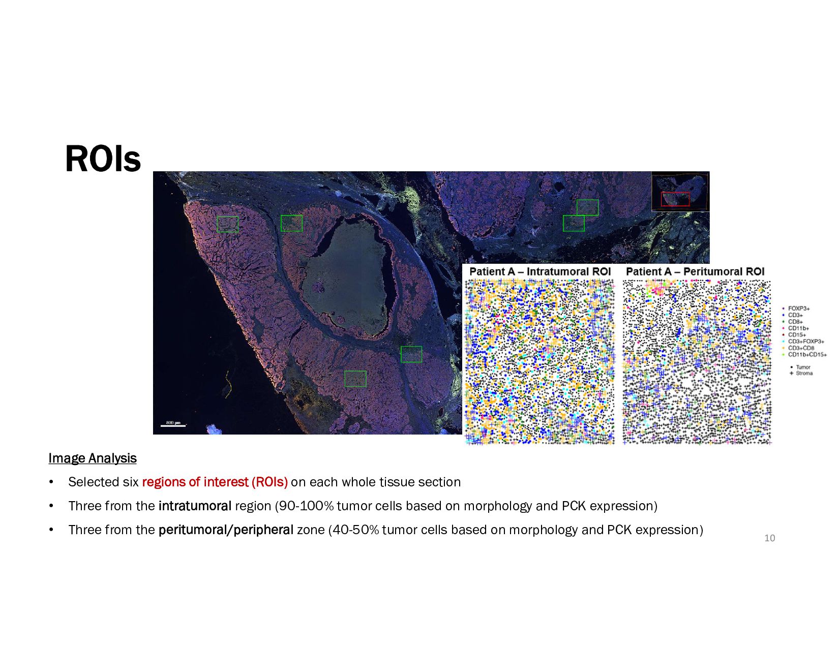
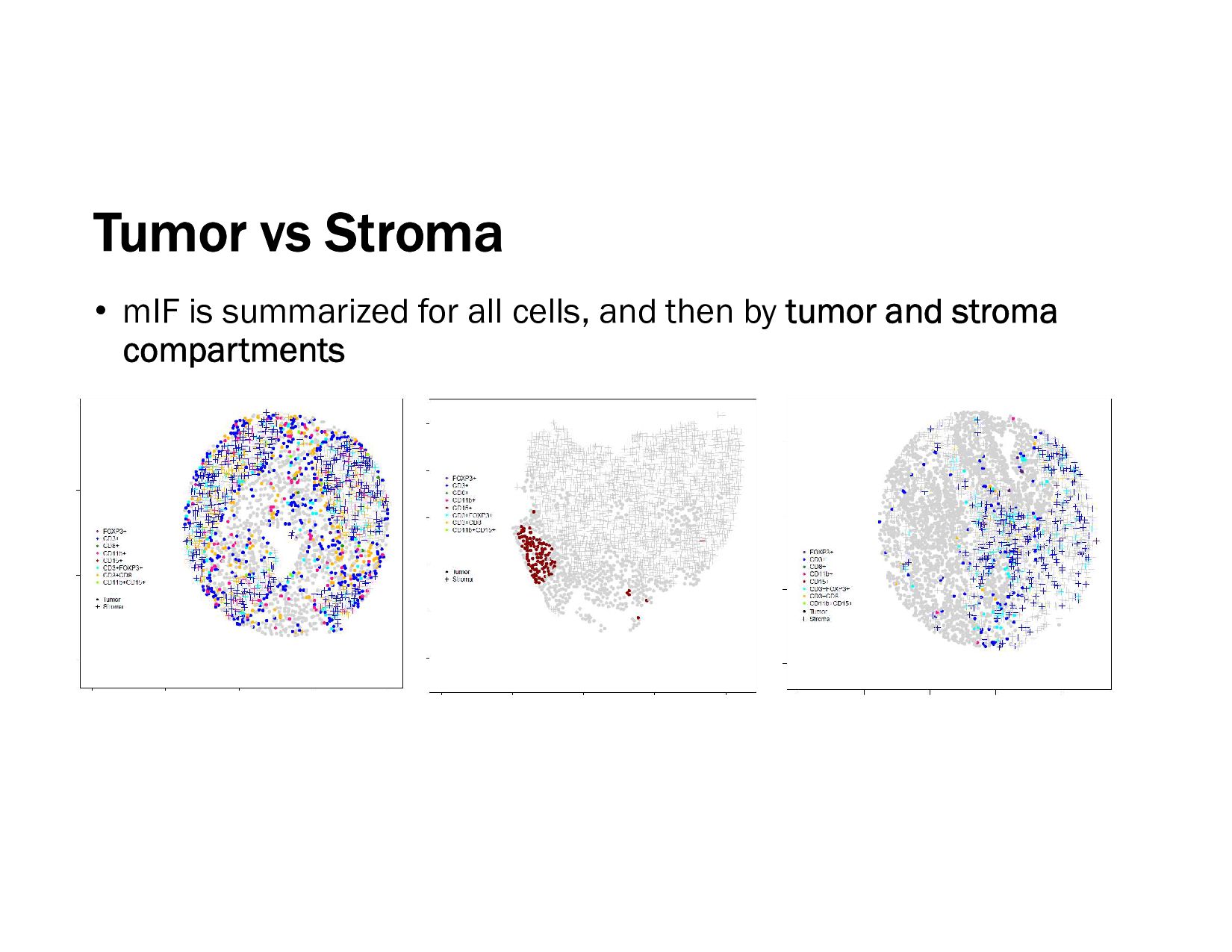
10. ROIs Image Analysis • Selected six regions of interest (ROIs) on each whole tissue section • Three from the intratumoral region (90-100% tumor cells based on morphology and PCK expression) • Three from the peritumoral/peripheral zone (40-50% tumor cells based on morphology and PCK expression) 10
11. Tumor vs Stroma • mIF is summarized for all cells, and then by tumor and stroma compartments
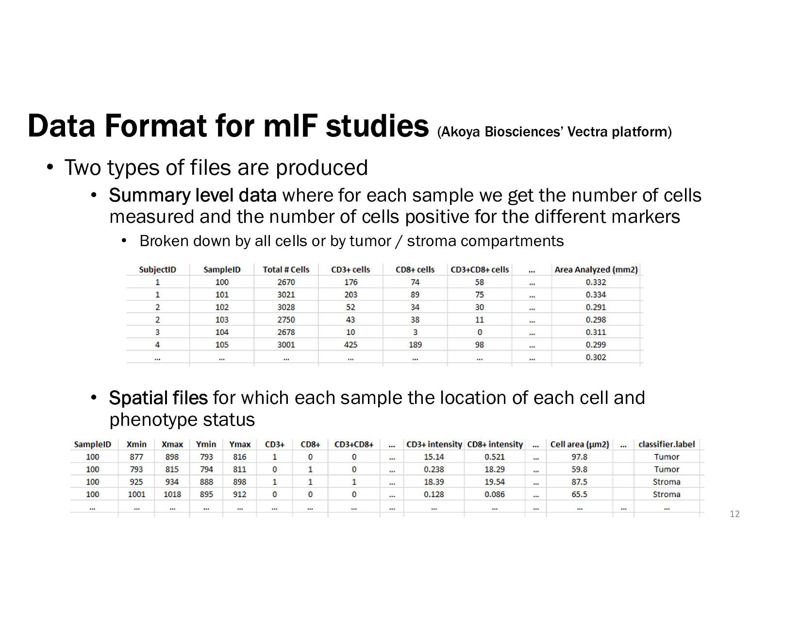
12. Data Format for mIF studies (Akoya Biosciences’ Vectra platform) • Two types of files are produced • Summary level data where for each sample we get the number of cells measured and the number of cells positive for the different markers • Broken down by all cells or by tumor / stroma compartments • Spatial files for which each sample the location of each cell and phenotype status 12
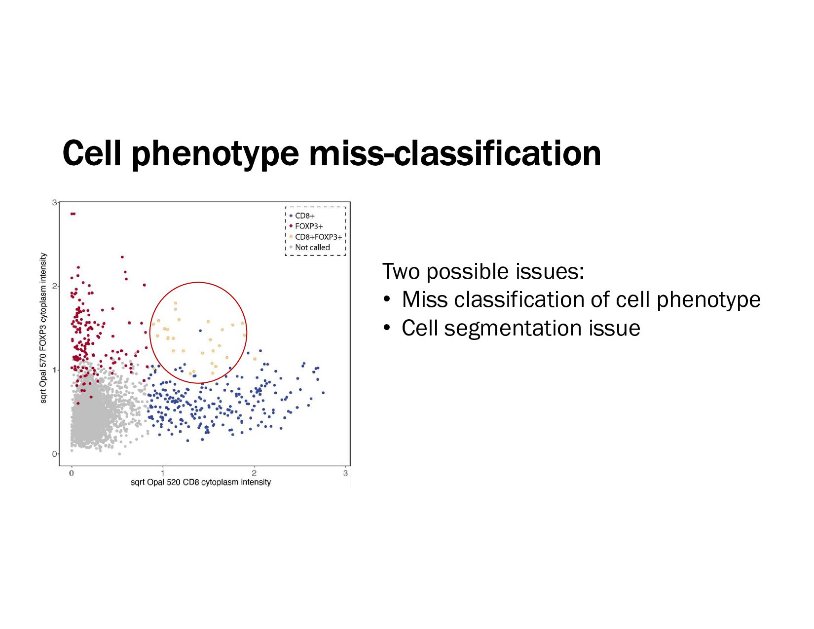
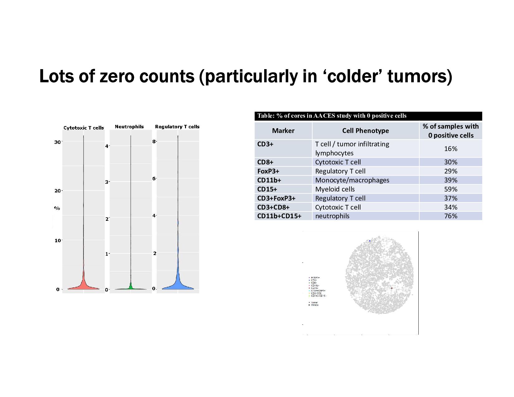
13. Challenges in analyses of mIF data • Quality Control • Mis-classification of cell type / phenotyping • Batch effects • Many zero count for cells positive for a marker • Zero-inflated or over-dispersed distribution • For spatial analysis of TMAs, areas of “missing cells” or “holes” • Repeated measurements per tumor/subject 13
14. Cell phenotype miss-classification Two possible issues: • Miss classification of cell phenotype • Cell segmentation issue
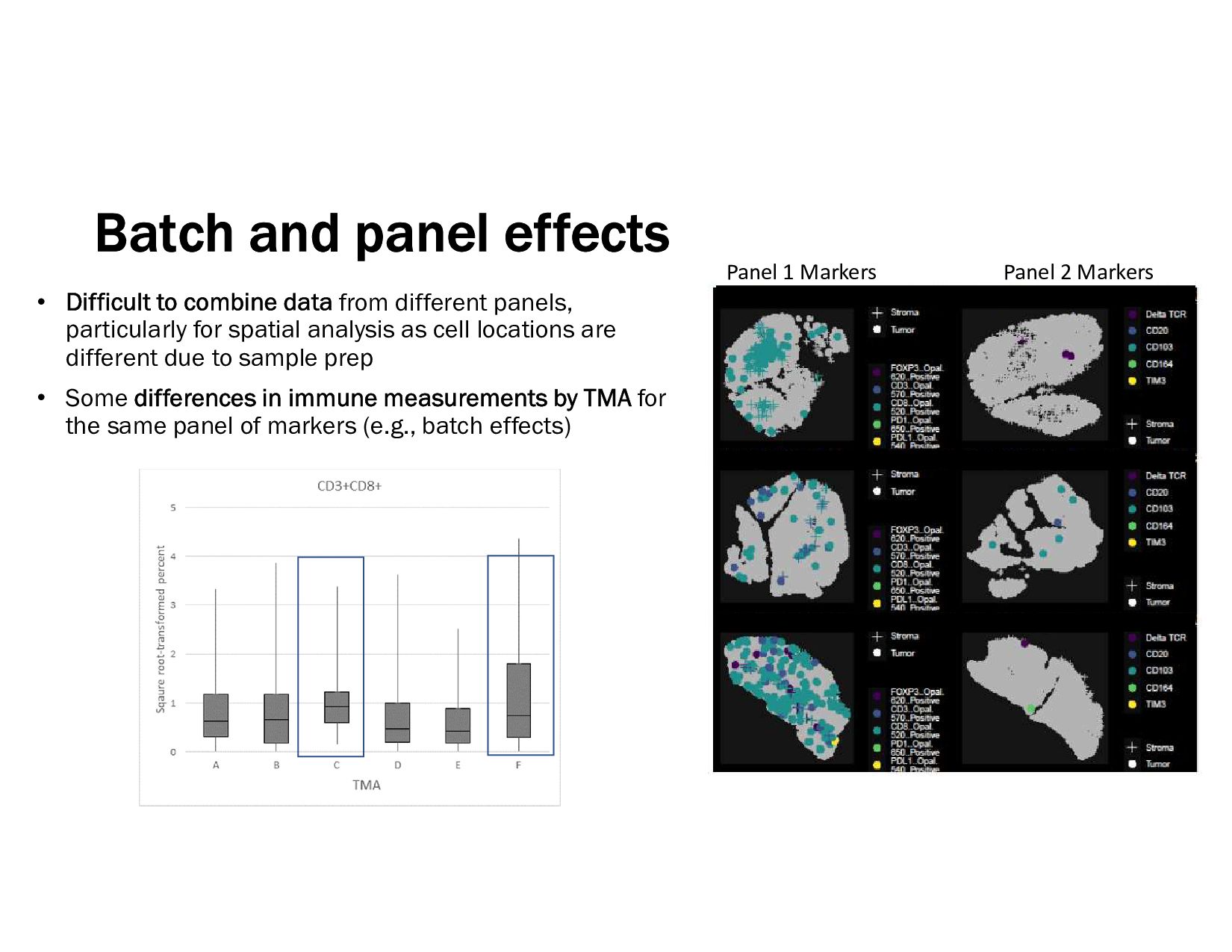
15. Batch and panel effects • Difficult to combine data from different panels, particularly for spatial analysis as cell locations are different due to sample prep • Some differences in immune measurements by TMA for the same panel of markers (e.g., batch effects) Panel 1 Markers Panel 2 Markers
16. Lots of zero counts (particularly in ‘colder’ tumors) Table: % of cores in AACES study with 0 positive cells Marker Cell Phenotype % of samples with 0 positive cells CD3+ T cell / tumor infiltrating lymphocytes 16% CD8+ Cytotoxic T cell 30% FoxP3+ Regulatory T cell 29% CD11b+ Monocyte/macrophages 39% CD15+ Myeloid cells 59% CD3+FoxP3+ Regulatory T cell 37% CD3+CD8+ Cytotoxic T cell 34% CD11b+CD15+ neutrophils 76%
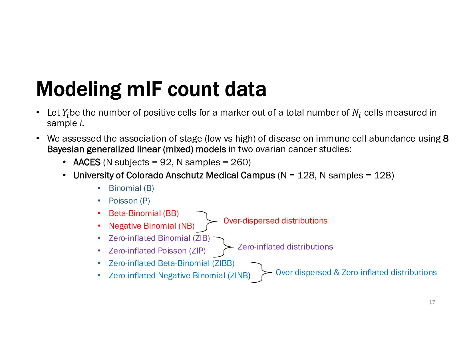
17. Modeling mIF count data • Let 𝑌 be the number of positive cells for a marker out of a total number of 𝑁 cells measured in sample i. • We assessed the association of stage (low vs high) of disease on immune cell abundance using 8 Bayesian generalized linear (mixed) models in two ovarian cancer studies: • AACES (N subjects = 92, N samples = 260) • University of Colorado Anschutz Medical Campus (N = 128, N samples = 128) • Binomial (B) • Poisson (P) • Beta-Binomial (BB) • Negative Binomial (NB) • Zero-inflated Binomial (ZIB) • Zero-inflated Poisson (ZIP) • Zero-inflated Beta-Binomial (ZIBB) • Zero-inflated Negative Binomial (ZINB) 17 Over-dispersed distributions Zero-inflated distributions Over-dispersed & Zero-inflated distributions
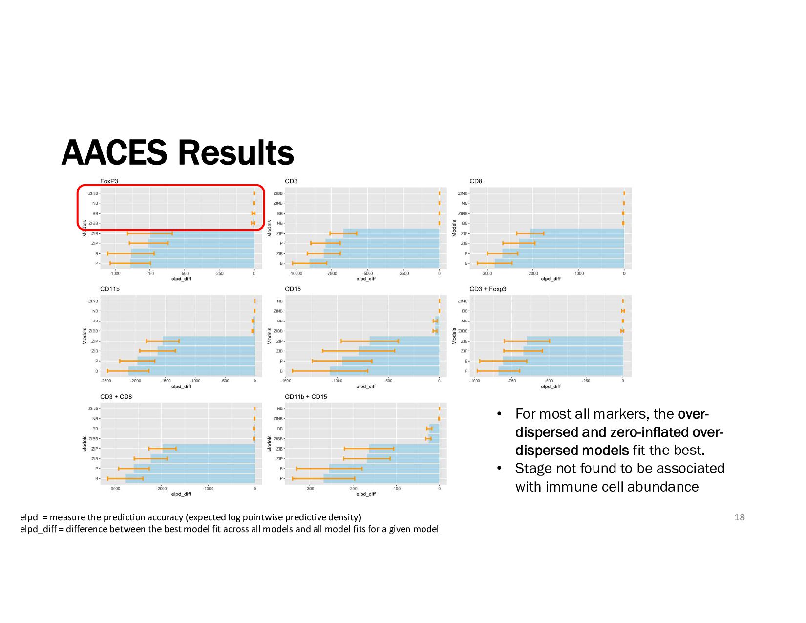
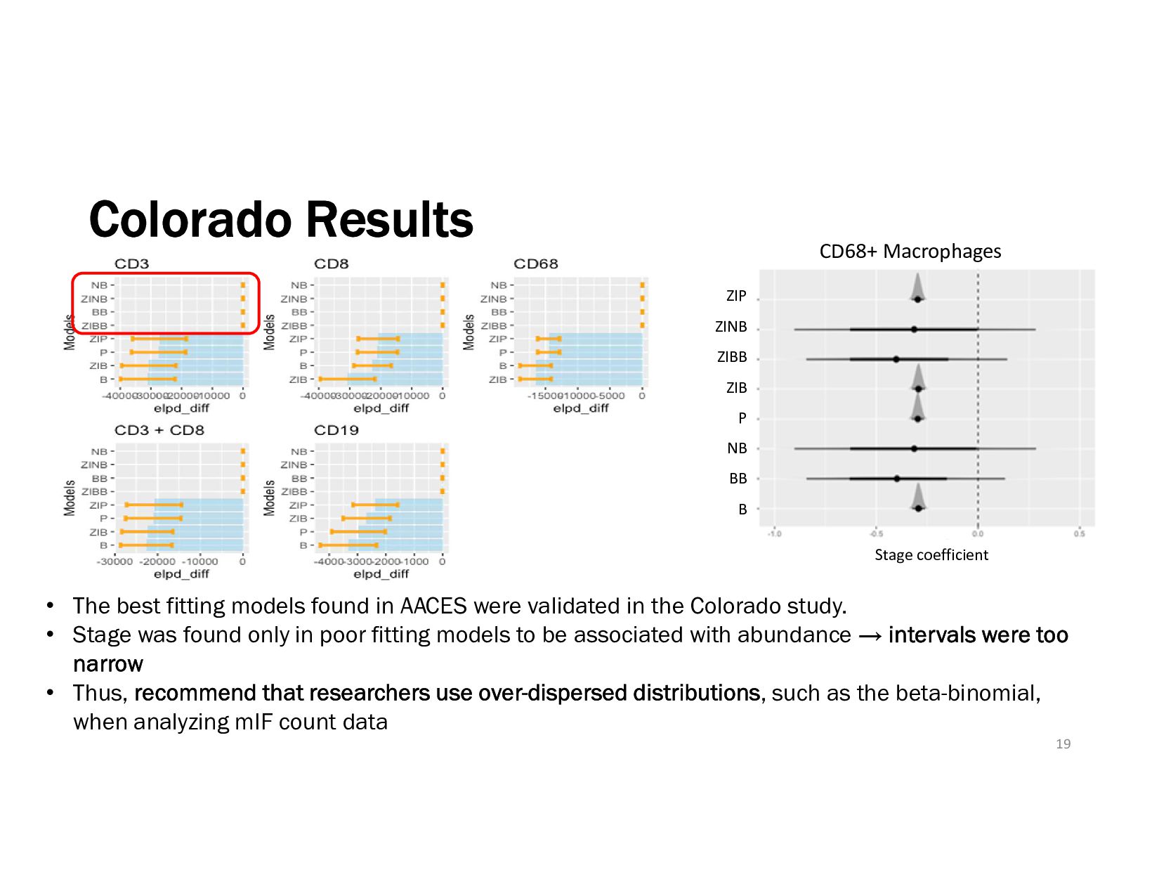
18. AACES Results 18 • For most all markers, the over- dispersed and zero-inflated over- dispersed models fit the best. • Stage not found to be associated with immune cell abundance elpd = measure the prediction accuracy (expected log pointwise predictive density) elpd_diff = difference between the best model fit across all models and all model fits for a given model
19. Colorado Results 19 • The best fitting models found in AACES were validated in the Colorado study. • Stage was found only in poor fitting models to be associated with abundance → intervals were too narrow • Thus, recommend that researchers use over-dispersed distributions, such as the beta-binomial, when analyzing mIF count data CD68+ Macrophages Stage coefficient ZIP ZINB ZIBB ZIB P NB BB B
20. Spatial clustering of different cell types 20
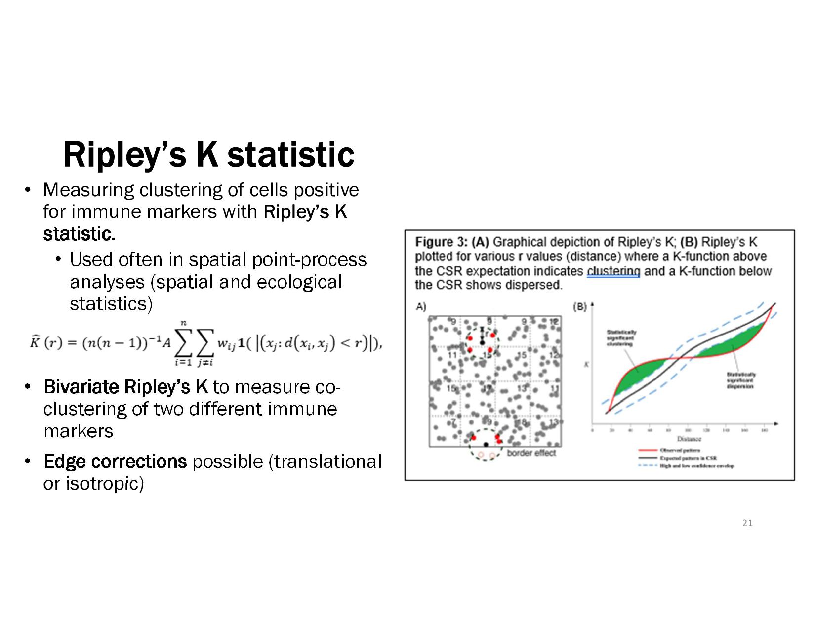
21. Ripley’s K statistic • Measuring clustering of cells positive for immune markers with Ripley’s K statistic. • Used often in spatial point-process analyses (spatial and ecological statistics) • Bivariate Ripley’s K to measure co- clustering of two different immune markers • Edge corrections possible (translational or isotropic) 21
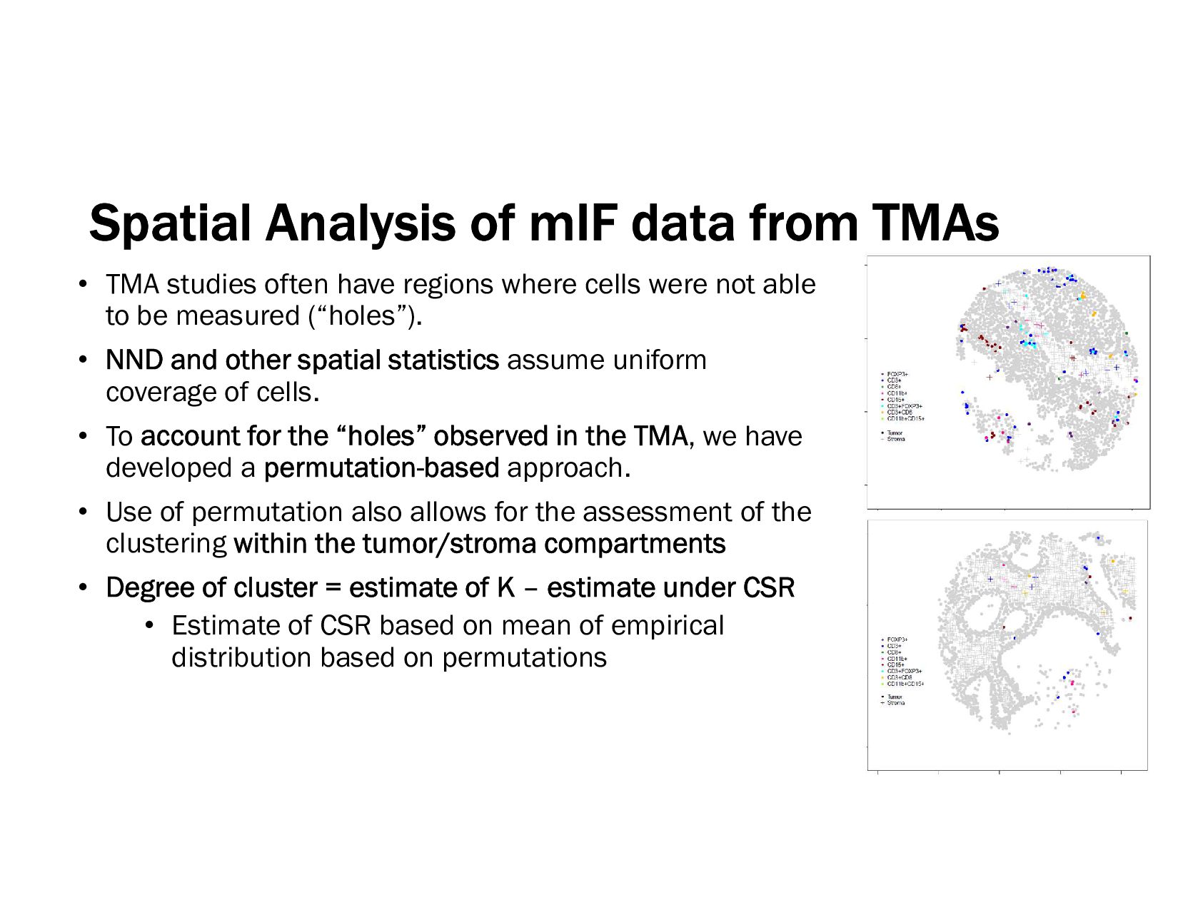
22. Spatial Analysis of mIF data from TMAs • TMA studies often have regions where cells were not able to be measured (“holes”). • NND and other spatial statistics assume uniform coverage of cells. • To account for the “holes” observed in the TMA, we have developed a permutation-based approach. • Use of permutation also allows for the assessment of the clustering within the tumor/stroma compartments • Degree of cluster = estimate of K – estimate under CSR • Estimate of CSR based on mean of empirical distribution based on permutations 22
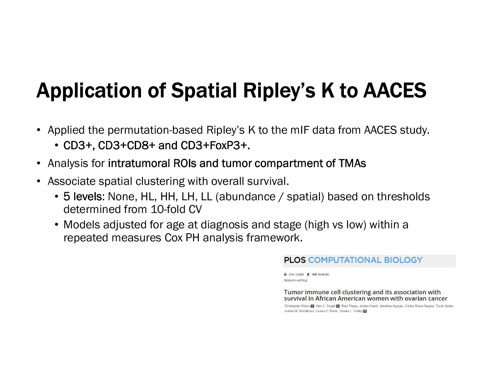
23. Application of Spatial Ripley’s K to AACES • Applied the permutation-based Ripley’s K to the mIF data from AACES study. • CD3+, CD3+CD8+ and CD3+FoxP3+. • Analysis for intratumoral ROIs and tumor compartment of TMAs • Associate spatial clustering with overall survival. • 5 levels: None, HL, HH, LH, LL (abundance / spatial) based on thresholds determined from 10-fold CV • Models adjusted for age at diagnosis and stage (high vs low) within a repeated measures Cox PH analysis framework. 23
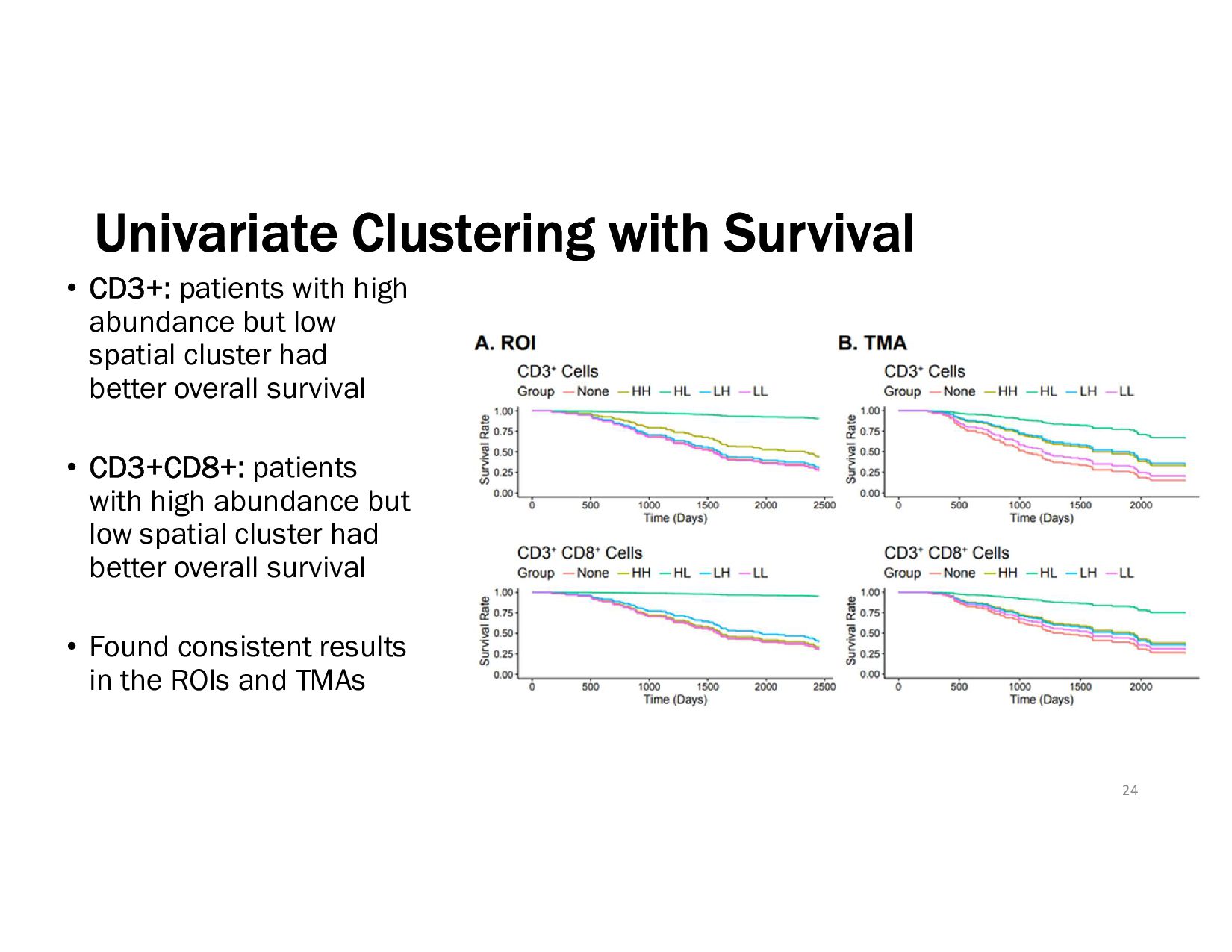
24. Univariate Clustering with Survival • CD3+: patients with high abundance but low spatial cluster had better overall survival • CD3+CD8+: patients with high abundance but low spatial cluster had better overall survival • Found consistent results in the ROIs and TMAs 24
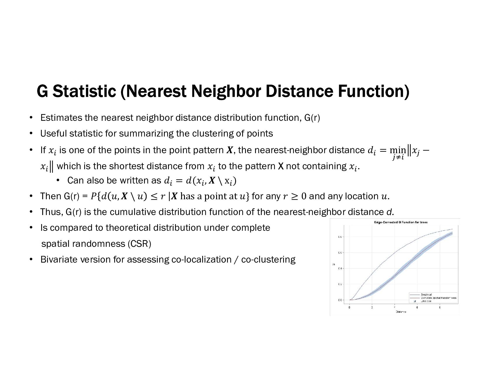
25. G Statistic (Nearest Neighbor Distance Function) • Estimates the nearest neighbor distance distribution function, G(r) • Useful statistic for summarizing the clustering of points • If 𝑥 is one of the points in the point pattern 𝑿, the nearest-neighbor distance 𝑑 = min 𝑥 − 𝑥 which is the shortest distance from 𝑥 to the pattern X not containing 𝑥 . • Can also be written as 𝑑 = 𝑑(𝑥 , 𝑿 \ x ) • Then G(r) = 𝑃 𝑑 𝑢, 𝑿 \ 𝑢 ≤ 𝑟 𝑿 has a point at 𝑢} for any 𝑟 ≥ 0 and any location 𝑢. • Thus, G(r) is the cumulative distribution function of the nearest-neighbor distance d. • Is compared to theoretical distribution under complete spatial randomness (CSR) • Bivariate version for assessing co-localization / co-clustering 25
26. Steinhart et al (2021) interaction variable 26
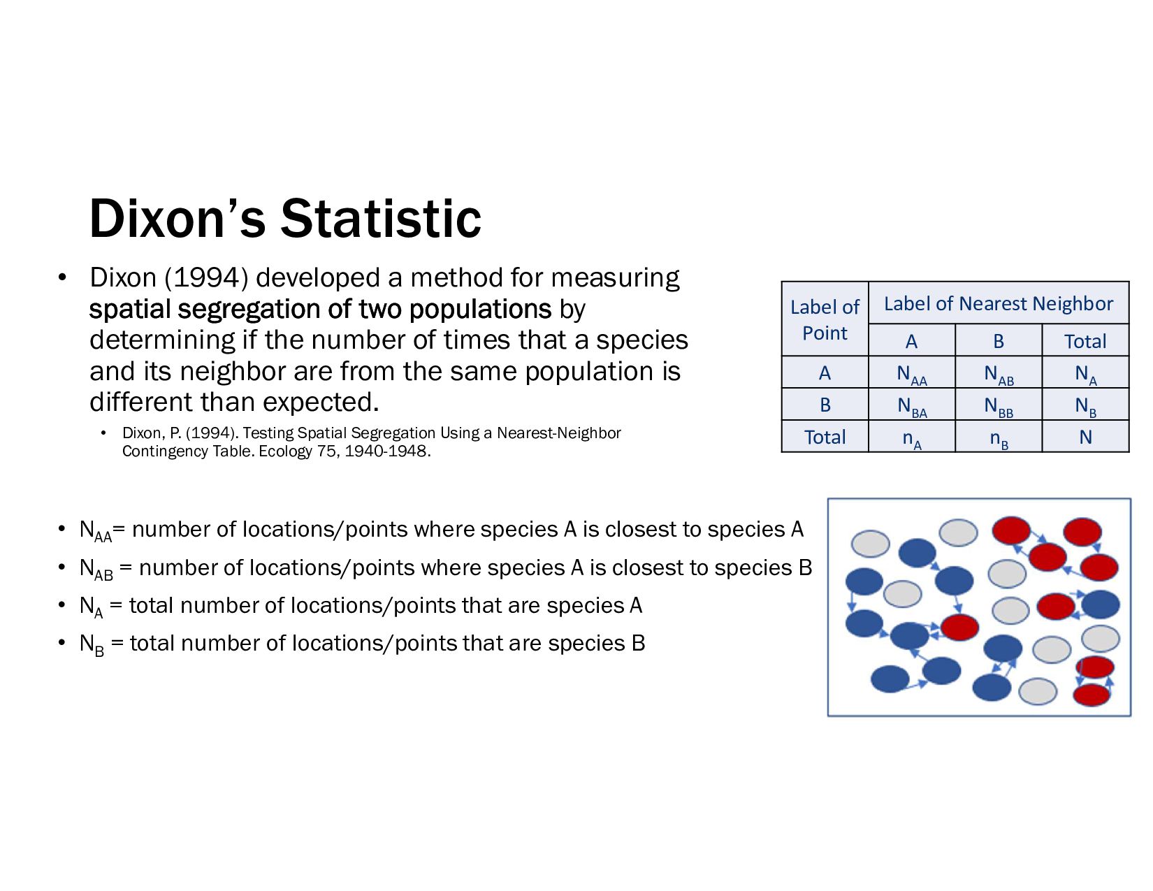
27. Dixon’s Statistic • Dixon (1994) developed a method for measuring spatial segregation of two populations by determining if the number of times that a species and its neighbor are from the same population is different than expected. • Dixon, P. (1994). Testing Spatial Segregation Using a Nearest-Neighbor Contingency Table. Ecology 75, 1940-1948. • NAA = number of locations/points where species A is closest to species A • NAB = number of locations/points where species A is closest to species B • NA = total number of locations/points that are species A • NB = total number of locations/points that are species B Label of Point Label of Nearest Neighbor A B Total A NAA NAB NA B NBA NBB NB Total nA nB N
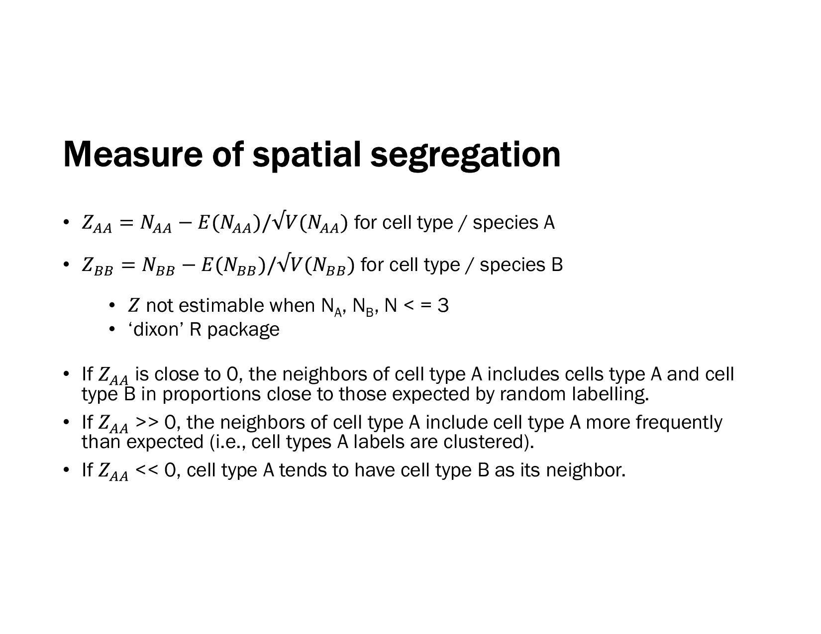
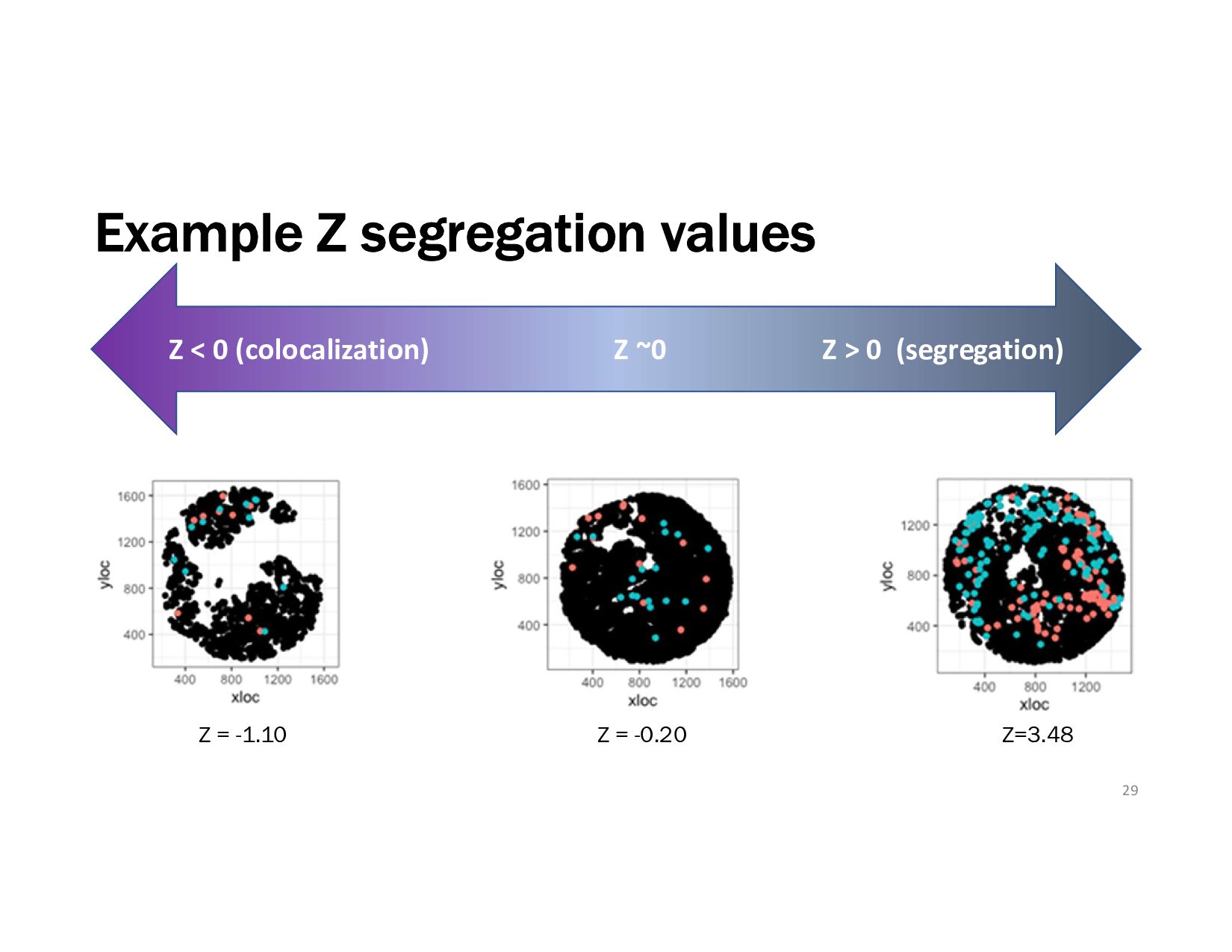
28. Measure of spatial segregation • for cell type / species A • for cell type / species B • not estimable when NA , NB , N < = 3 • ‘dixon’ R package • If is close to 0, the neighbors of cell type A includes cells type A and cell type B in proportions close to those expected by random labelling. • If >> 0, the neighbors of cell type A include cell type A more frequently than expected (i.e., cell types A labels are clustered). • If << 0, cell type A tends to have cell type B as its neighbor.
29. Example Z segregation values 29 Z < 0 (colocalization) Z ~0 Z > 0 (segregation) Z = -1.10 Z = -0.20 Z=3.48
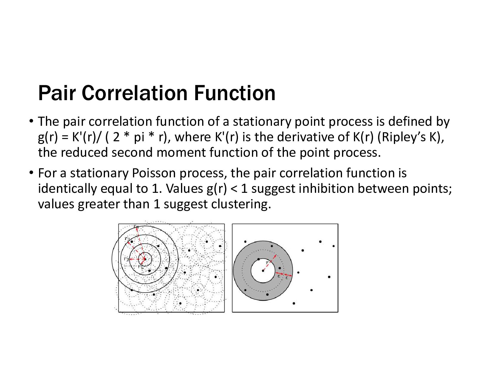
30. Pair Correlation Function • The pair correlation function of a stationary point process is defined by g(r) = K'(r)/ ( 2 * pi * r), where K'(r) is the derivative of K(r) (Ripley’s K), the reduced second moment function of the point process. • For a stationary Poisson process, the pair correlation function is identically equal to 1. Values g(r) < 1 suggest inhibition between points; values greater than 1 suggest clustering.
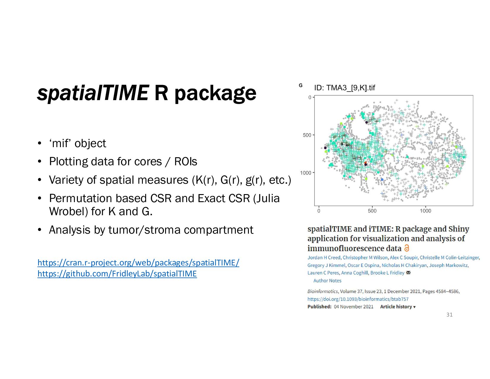
31. spatialTIME R package • ‘mif’ object • Plotting data for cores / ROIs • Variety of spatial measures (K(r), G(r), g(r), etc.) • Permutation based CSR and Exact CSR (Julia Wrobel) for K and G. • Analysis by tumor/stroma compartment 31 https://cran.r-project.org/web/packages/spatialTIME/ https://github.com/FridleyLab/spatialTIME
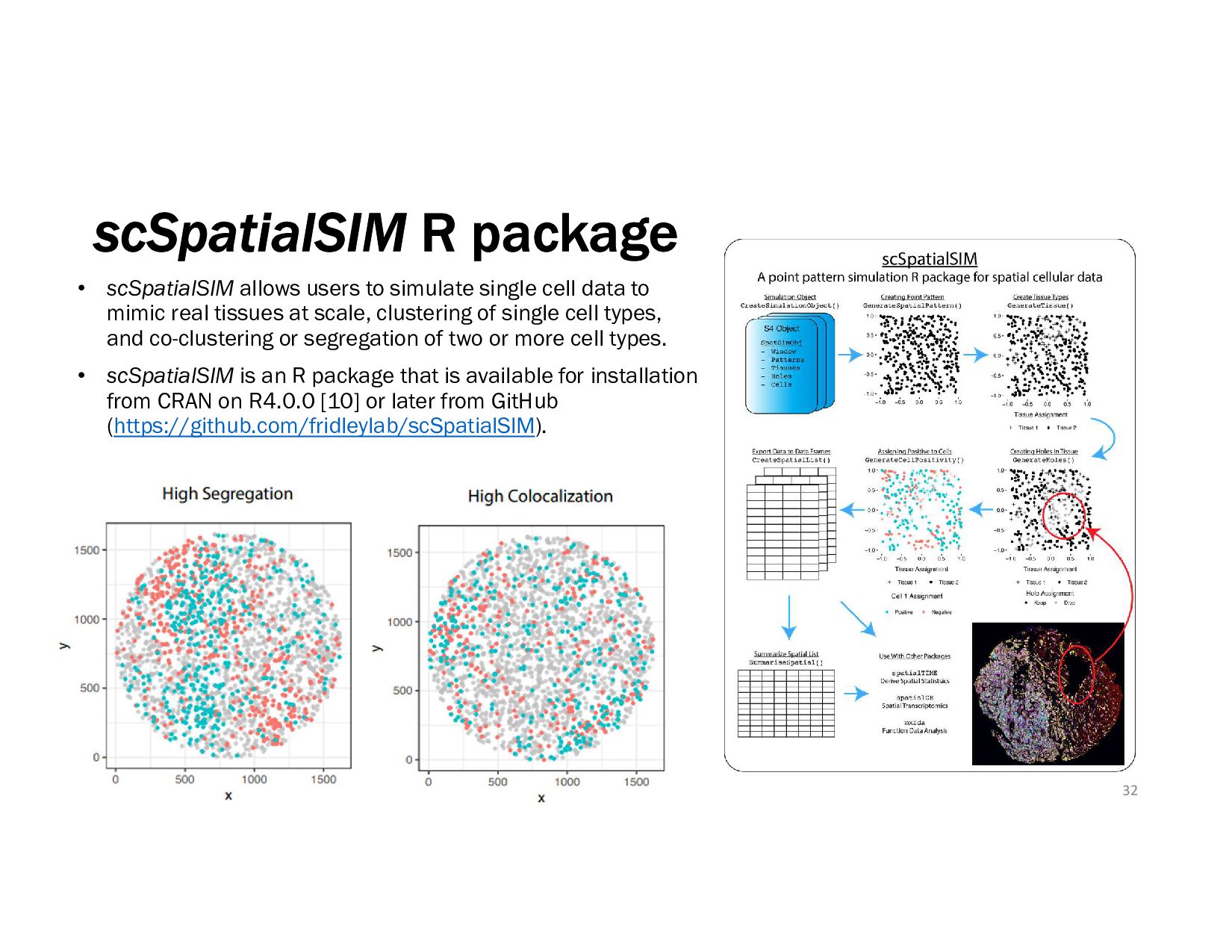
32. scSpatialSIM R package • scSpatialSIM allows users to simulate single cell data to mimic real tissues at scale, clustering of single cell types, and co-clustering or segregation of two or more cell types. • scSpatialSIM is an R package that is available for installation from CRAN on R4.0.0 [10] or later from GitHub (https://github.com/fridleylab/scSpatialSIM). 32
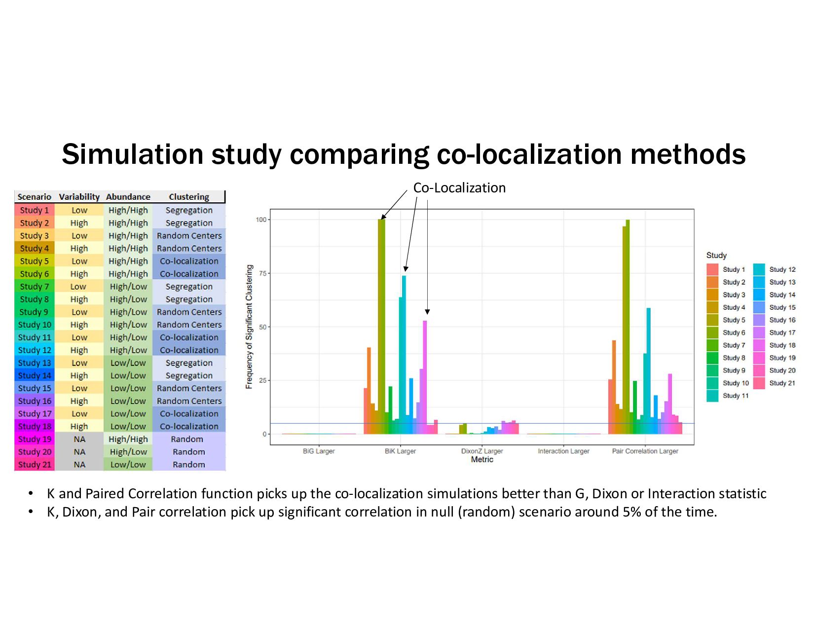
33. Simulation study comparing co-localization methods • K and Paired Correlation function picks up the co-localization simulations better than G, Dixon or Interaction statistic • K, Dixon, and Pair correlation pick up significant correlation in null (random) scenario around 5% of the time. Co-Localization
34. Comparison of 5 Co-localization Methods in 5 Ovarian Cancer Studies of Cytotoxic T-cells (CD8+) and Regulatory T-Cells (FoxP3+) 34
35. Acknowledgements • Alex Soupir • Chris Wilson • Oscar Ospina • Lauren C Peres • Christelle Colin-Leitzinger • Joellen M Schildkraut • Jordan Creed • Ben Bitler • Julia Wrobel • Katie Terry • Shelley Tworoger • Mary Townsend • Andrew Lawson 35 NIH R01 CA279065 (Fridley / Peres)