CAIP 2013

Patch Blending

Transcript

1. Spatial Patch Blending for Patch-based Inpainting Methods Maxime Daisy, David Tschumperl´ e, Olivier L´ ezoray GREYC, CRNS UMR 6072 ´ Equipe Image - ENSICAEN 6, boulevard du Mar´ echal Juin 14050 Caen cedex {maxime.daisy, david.tschumperle, olivier.lezoray}@ensicaen.fr 20th of June, 2013
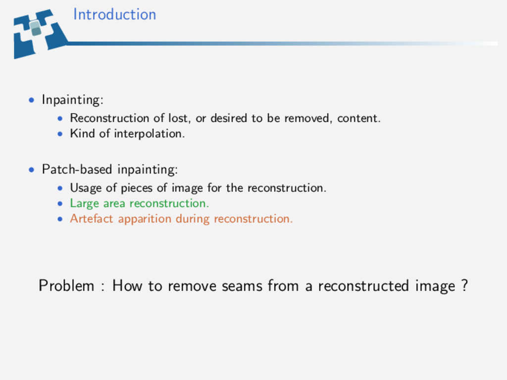
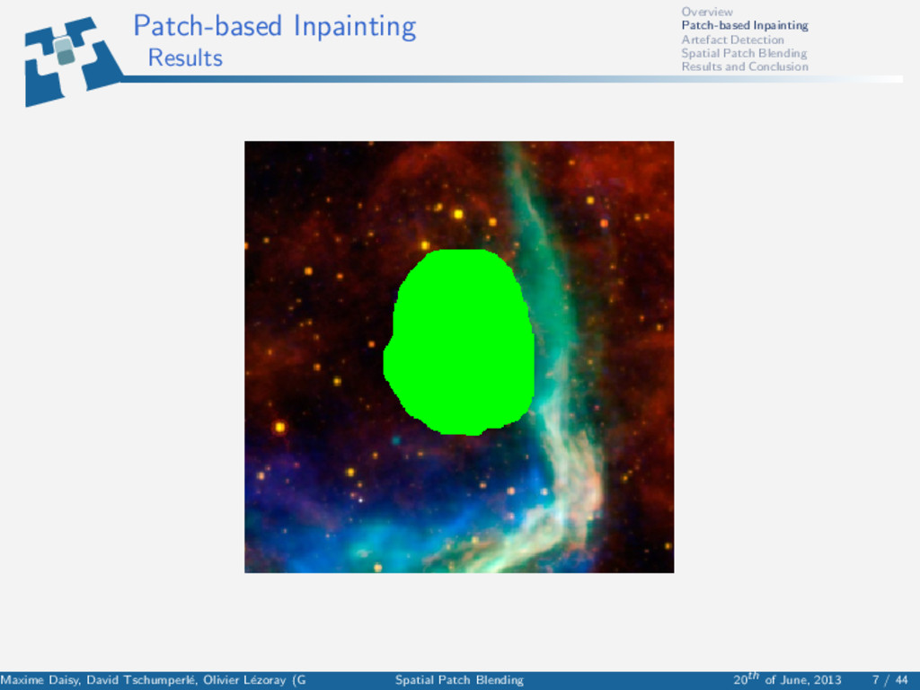
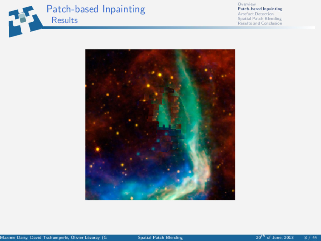
2. Introduction • Inpainting: • Reconstruction of lost, or desired to be removed, content. • Kind of interpolation. • Patch-based inpainting: • Usage of pieces of image for the reconstruction. • Large area reconstruction. • Artefact apparition during reconstruction. Problem : How to remove seams from a reconstructed image ?
3. Overview Patch-based Inpainting Artefact Detection Spatial Patch Blending Results and Conclusion Overview 1 Patch-based Inpainting Entry-level Algorithm Method Results 2 Artefact Detection Principle Break Detection Process 3 Spatial Patch Blending Principle in four images Two Methods Blend Scales Optimisation 4 Results and Conclusion Maxime Daisy, David Tschumperl´ e, Olivier L´ ezoray (GREYC) Spatial Patch Blending 20th of June, 2013 3 / 44
4. Overview Patch-based Inpainting Artefact Detection Spatial Patch Blending Results and Conclusion Patch-based Inpainting Entry-level Algorithm [?] Maxime Daisy, David Tschumperl´ e, Olivier L´ ezoray (GREYC) Spatial Patch Blending 20th of June, 2013 4 / 44
5. Overview Patch-based Inpainting Artefact Detection Spatial Patch Blending Results and Conclusion Patch-based Inpainting Results Maxime Daisy, David Tschumperl´ e, Olivier L´ ezoray (GREYC) Spatial Patch Blending 20th of June, 2013 5 / 44
6. Overview Patch-based Inpainting Artefact Detection Spatial Patch Blending Results and Conclusion Patch-based Inpainting Results Maxime Daisy, David Tschumperl´ e, Olivier L´ ezoray (GREYC) Spatial Patch Blending 20th of June, 2013 6 / 44
7. Overview Patch-based Inpainting Artefact Detection Spatial Patch Blending Results and Conclusion Patch-based Inpainting Results Maxime Daisy, David Tschumperl´ e, Olivier L´ ezoray (GREYC) Spatial Patch Blending 20th of June, 2013 7 / 44
8. Overview Patch-based Inpainting Artefact Detection Spatial Patch Blending Results and Conclusion Patch-based Inpainting Results Maxime Daisy, David Tschumperl´ e, Olivier L´ ezoray (GREYC) Spatial Patch Blending 20th of June, 2013 8 / 44
9. Overview Patch-based Inpainting Artefact Detection Spatial Patch Blending Results and Conclusion Patch-based Inpainting Results Maxime Daisy, David Tschumperl´ e, Olivier L´ ezoray (GREYC) Spatial Patch Blending 20th of June, 2013 9 / 44
10. Overview Patch-based Inpainting Artefact Detection Spatial Patch Blending Results and Conclusion Patch-based Inpainting Results Maxime Daisy, David Tschumperl´ e, Olivier L´ ezoray (GREYC) Spatial Patch Blending 20th of June, 2013 10 / 44
11. Overview Patch-based Inpainting Artefact Detection Spatial Patch Blending Results and Conclusion Artefact Detection Principle 3 steps enclosed under Artefact detection word : 1 Breaks detection. ⇒ location of image singularities. 2 Strongest break points extraction. ⇒ break field thresholding. 3 Blending amplitude field generation σ. ⇒ one input of the spatial patch blending algorithm. Maxime Daisy, David Tschumperl´ e, Olivier L´ ezoray (GREYC) Spatial Patch Blending 20th of June, 2013 11 / 44
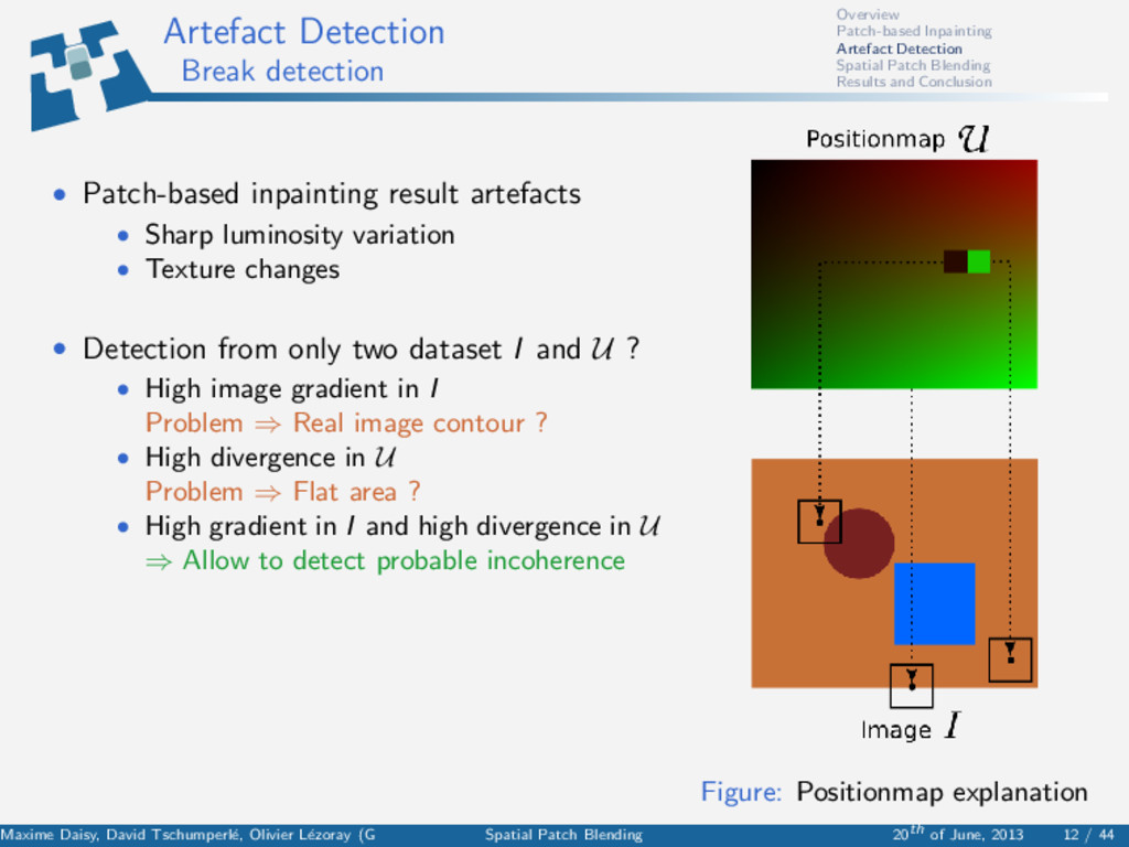
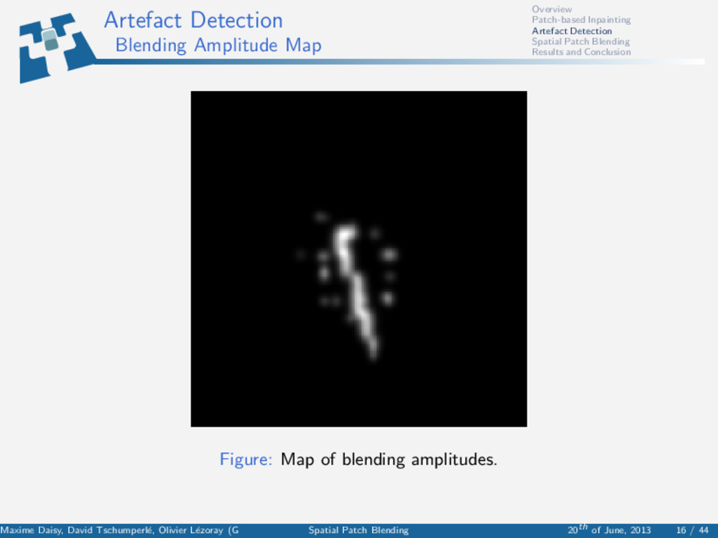
12. Overview Patch-based Inpainting Artefact Detection Spatial Patch Blending Results and Conclusion Artefact Detection Break detection • Patch-based inpainting result artefacts • Sharp luminosity variation • Texture changes • Detection from only two dataset I and U ? • High image gradient in I Problem ⇒ Real image contour ? • High divergence in U Problem ⇒ Flat area ? • High gradient in I and high divergence in U ⇒ Allow to detect probable incoherence Figure: Positionmap explanation Maxime Daisy, David Tschumperl´ e, Olivier L´ ezoray (GREYC) Spatial Patch Blending 20th of June, 2013 12 / 44
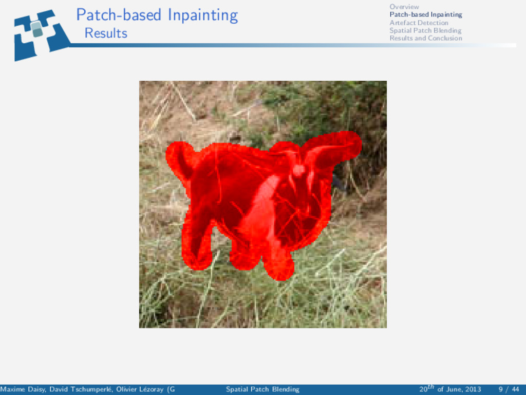
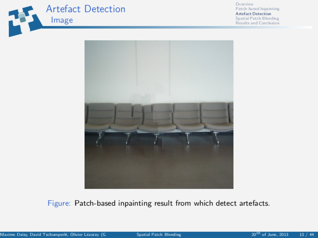
13. Overview Patch-based Inpainting Artefact Detection Spatial Patch Blending Results and Conclusion Artefact Detection Image Figure: Patch-based inpainting result from which detect artefacts. Maxime Daisy, David Tschumperl´ e, Olivier L´ ezoray (GREYC) Spatial Patch Blending 20th of June, 2013 13 / 44
14. Overview Patch-based Inpainting Artefact Detection Spatial Patch Blending Results and Conclusion Artefact Detection Break field Figure: Break field. Maxime Daisy, David Tschumperl´ e, Olivier L´ ezoray (GREYC) Spatial Patch Blending 20th of June, 2013 14 / 44
15. Overview Patch-based Inpainting Artefact Detection Spatial Patch Blending Results and Conclusion Artefact Detection Break points Figure: Break points. Maxime Daisy, David Tschumperl´ e, Olivier L´ ezoray (GREYC) Spatial Patch Blending 20th of June, 2013 15 / 44
16. Overview Patch-based Inpainting Artefact Detection Spatial Patch Blending Results and Conclusion Artefact Detection Blending Amplitude Map Figure: Map of blending amplitudes. Maxime Daisy, David Tschumperl´ e, Olivier L´ ezoray (GREYC) Spatial Patch Blending 20th of June, 2013 16 / 44
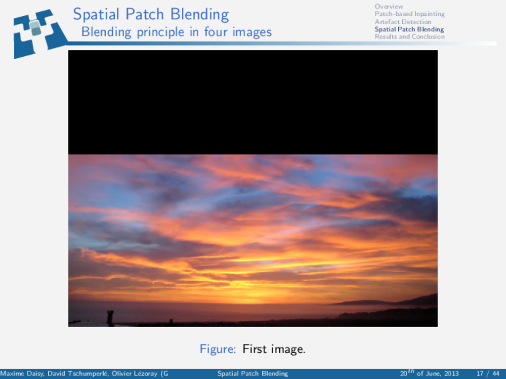
17. Overview Patch-based Inpainting Artefact Detection Spatial Patch Blending Results and Conclusion Spatial Patch Blending Blending principle in four images Figure: First image. Maxime Daisy, David Tschumperl´ e, Olivier L´ ezoray (GREYC) Spatial Patch Blending 20th of June, 2013 17 / 44
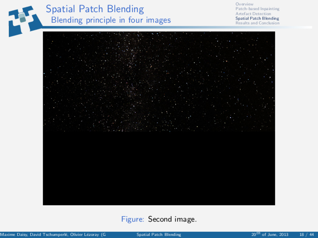
18. Overview Patch-based Inpainting Artefact Detection Spatial Patch Blending Results and Conclusion Spatial Patch Blending Blending principle in four images Figure: Second image. Maxime Daisy, David Tschumperl´ e, Olivier L´ ezoray (GREYC) Spatial Patch Blending 20th of June, 2013 18 / 44
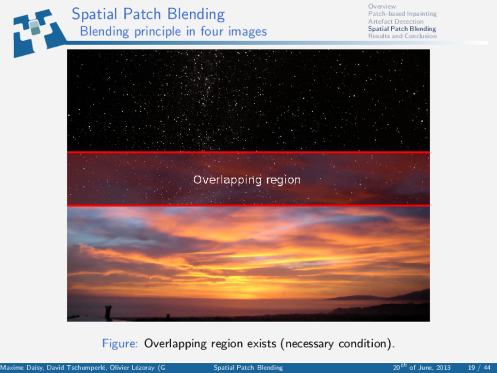
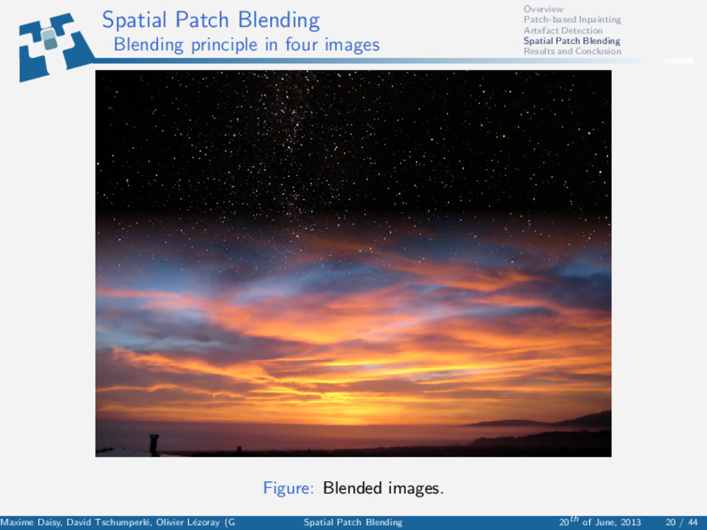
19. Overview Patch-based Inpainting Artefact Detection Spatial Patch Blending Results and Conclusion Spatial Patch Blending Blending principle in four images Figure: Overlapping region exists (necessary condition). Maxime Daisy, David Tschumperl´ e, Olivier L´ ezoray (GREYC) Spatial Patch Blending 20th of June, 2013 19 / 44
20. Overview Patch-based Inpainting Artefact Detection Spatial Patch Blending Results and Conclusion Spatial Patch Blending Blending principle in four images Figure: Blended images. Maxime Daisy, David Tschumperl´ e, Olivier L´ ezoray (GREYC) Spatial Patch Blending 20th of June, 2013 20 / 44
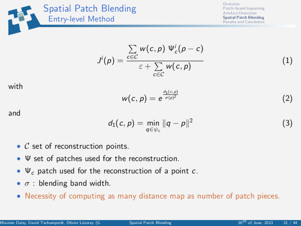
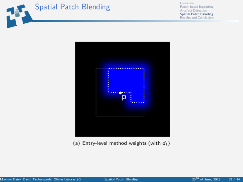
21. Overview Patch-based Inpainting Artefact Detection Spatial Patch Blending Results and Conclusion Spatial Patch Blending Entry-level Method Ji (p) = c∈C w(c, p) Ψi c (p − c) ε + c∈C w(c, p) (1) with w(c, p) = e d1(c,p) σ(p)2 (2) and d1 (c, p) = min q∈ψc q − p 2 (3) • C set of reconstruction points. • Ψ set of patches used for the reconstruction. • Ψc patch used for the reconstruction of a point c. • σ : blending band width. • Necessity of computing as many distance map as number of patch pieces. Maxime Daisy, David Tschumperl´ e, Olivier L´ ezoray (GREYC) Spatial Patch Blending 20th of June, 2013 21 / 44
22. Overview Patch-based Inpainting Artefact Detection Spatial Patch Blending Results and Conclusion Spatial Patch Blending (a) Entry-level method weights (with d1) Maxime Daisy, David Tschumperl´ e, Olivier L´ ezoray (GREYC) Spatial Patch Blending 20th of June, 2013 22 / 44
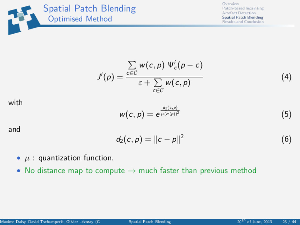
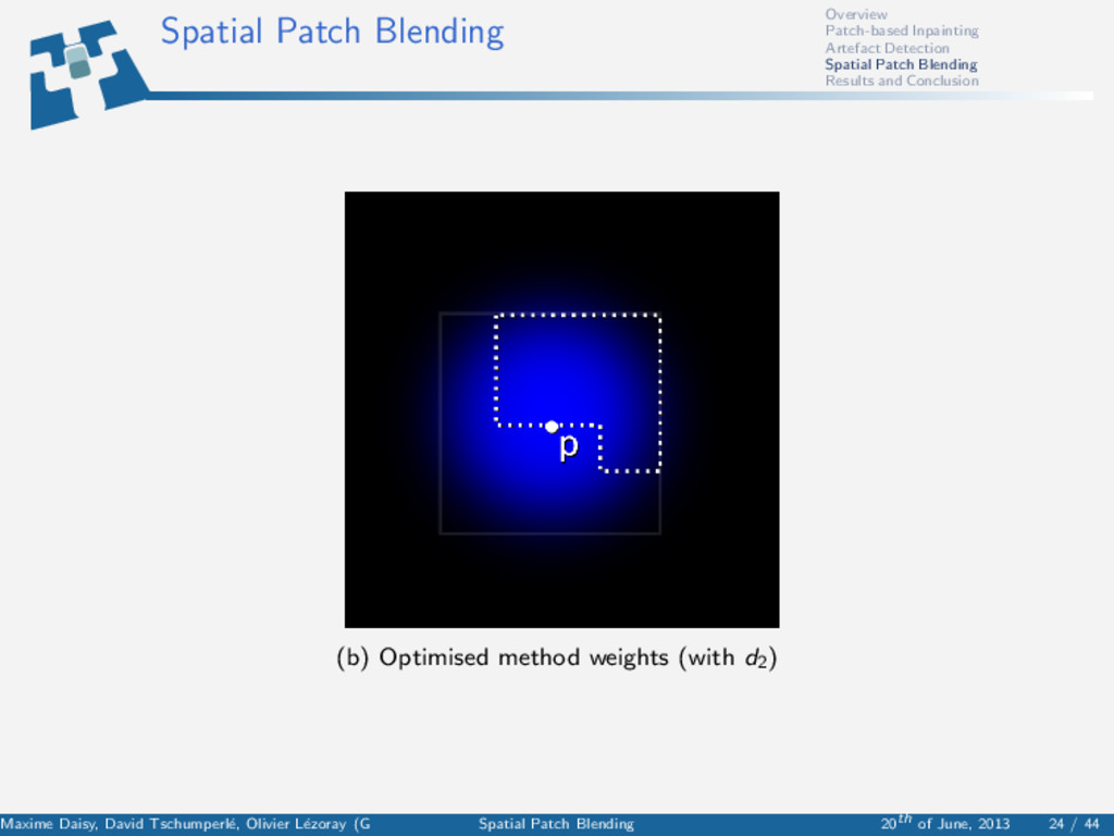
23. Overview Patch-based Inpainting Artefact Detection Spatial Patch Blending Results and Conclusion Spatial Patch Blending Optimised Method Ji (p) = c∈C w(c, p) Ψi c (p − c) ε + c∈C w(c, p) (4) with w(c, p) = e d2(c,p) µ(σ(p))2 (5) and d2 (c, p) = c − p 2 (6) • µ : quantization function. • No distance map to compute → much faster than previous method Maxime Daisy, David Tschumperl´ e, Olivier L´ ezoray (GREYC) Spatial Patch Blending 20th of June, 2013 23 / 44
24. Overview Patch-based Inpainting Artefact Detection Spatial Patch Blending Results and Conclusion Spatial Patch Blending (b) Optimised method weights (with d2) Maxime Daisy, David Tschumperl´ e, Olivier L´ ezoray (GREYC) Spatial Patch Blending 20th of June, 2013 24 / 44
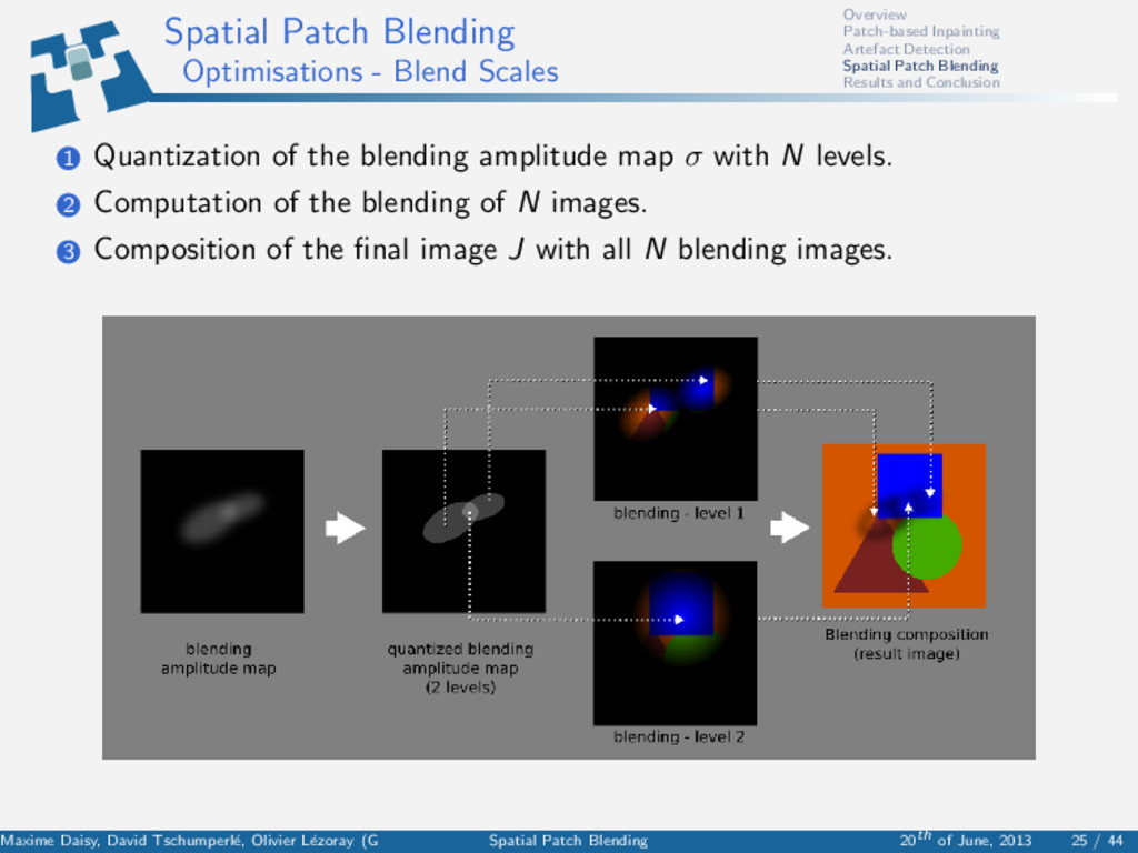
25. Overview Patch-based Inpainting Artefact Detection Spatial Patch Blending Results and Conclusion Spatial Patch Blending Optimisations - Blend Scales 1 Quantization of the blending amplitude map σ with N levels. 2 Computation of the blending of N images. 3 Composition of the final image J with all N blending images. Maxime Daisy, David Tschumperl´ e, Olivier L´ ezoray (GREYC) Spatial Patch Blending 20th of June, 2013 25 / 44
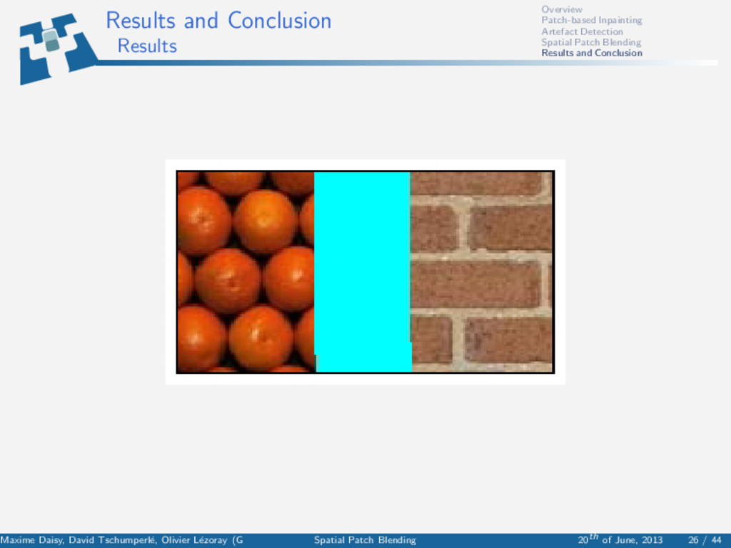
26. Overview Patch-based Inpainting Artefact Detection Spatial Patch Blending Results and Conclusion Results and Conclusion Results Maxime Daisy, David Tschumperl´ e, Olivier L´ ezoray (GREYC) Spatial Patch Blending 20th of June, 2013 26 / 44
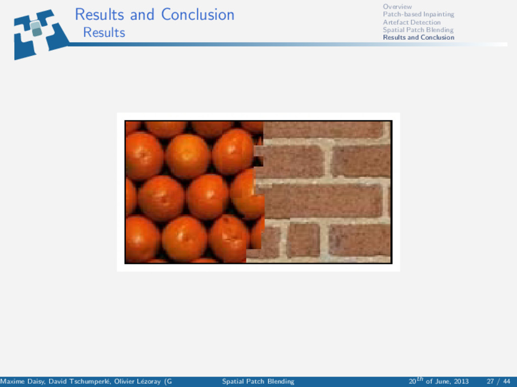
27. Overview Patch-based Inpainting Artefact Detection Spatial Patch Blending Results and Conclusion Results and Conclusion Results Maxime Daisy, David Tschumperl´ e, Olivier L´ ezoray (GREYC) Spatial Patch Blending 20th of June, 2013 27 / 44
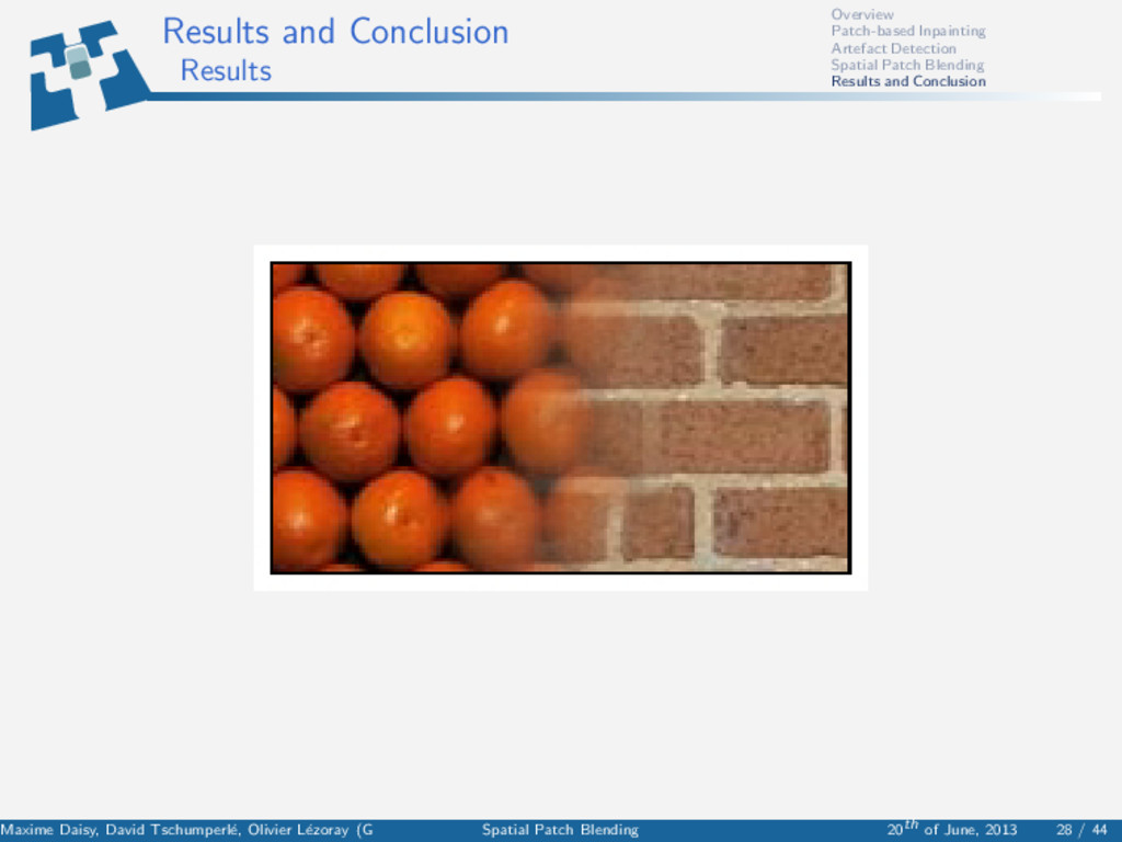
28. Overview Patch-based Inpainting Artefact Detection Spatial Patch Blending Results and Conclusion Results and Conclusion Results Maxime Daisy, David Tschumperl´ e, Olivier L´ ezoray (GREYC) Spatial Patch Blending 20th of June, 2013 28 / 44
29. Overview Patch-based Inpainting Artefact Detection Spatial Patch Blending Results and Conclusion Results and Conclusion Results Maxime Daisy, David Tschumperl´ e, Olivier L´ ezoray (GREYC) Spatial Patch Blending 20th of June, 2013 29 / 44
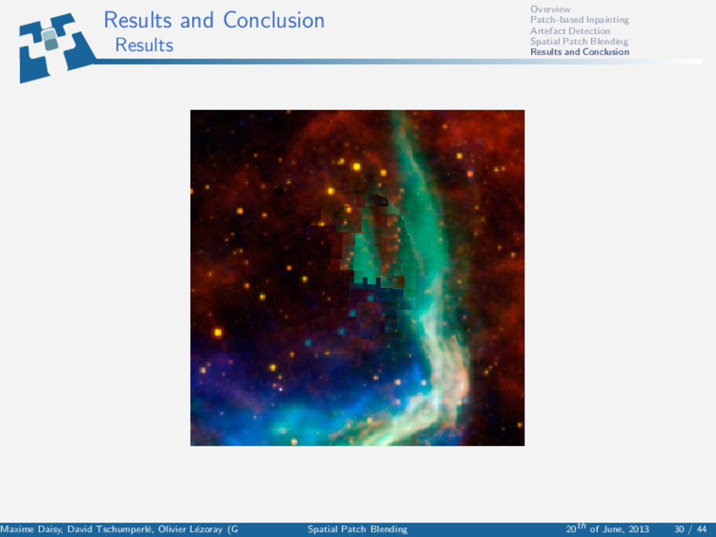
30. Overview Patch-based Inpainting Artefact Detection Spatial Patch Blending Results and Conclusion Results and Conclusion Results Maxime Daisy, David Tschumperl´ e, Olivier L´ ezoray (GREYC) Spatial Patch Blending 20th of June, 2013 30 / 44
31. Overview Patch-based Inpainting Artefact Detection Spatial Patch Blending Results and Conclusion Results and Conclusion Results Maxime Daisy, David Tschumperl´ e, Olivier L´ ezoray (GREYC) Spatial Patch Blending 20th of June, 2013 31 / 44
32. Overview Patch-based Inpainting Artefact Detection Spatial Patch Blending Results and Conclusion Results and Conclusion Results Maxime Daisy, David Tschumperl´ e, Olivier L´ ezoray (GREYC) Spatial Patch Blending 20th of June, 2013 32 / 44
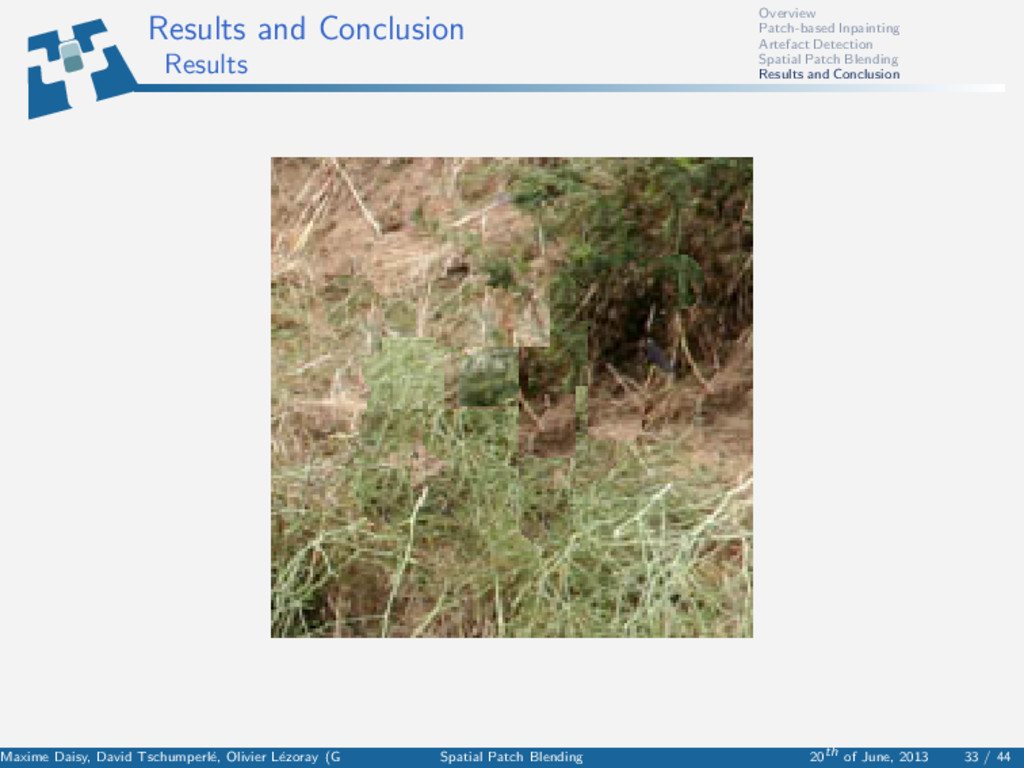
33. Overview Patch-based Inpainting Artefact Detection Spatial Patch Blending Results and Conclusion Results and Conclusion Results Maxime Daisy, David Tschumperl´ e, Olivier L´ ezoray (GREYC) Spatial Patch Blending 20th of June, 2013 33 / 44
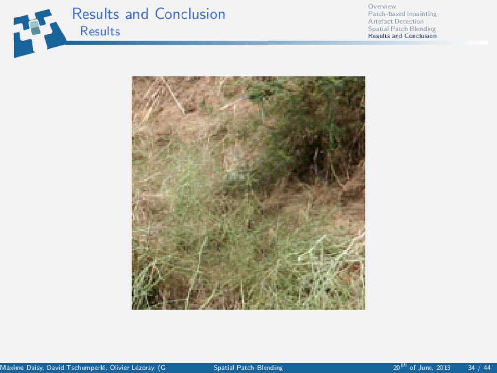
34. Overview Patch-based Inpainting Artefact Detection Spatial Patch Blending Results and Conclusion Results and Conclusion Results Maxime Daisy, David Tschumperl´ e, Olivier L´ ezoray (GREYC) Spatial Patch Blending 20th of June, 2013 34 / 44
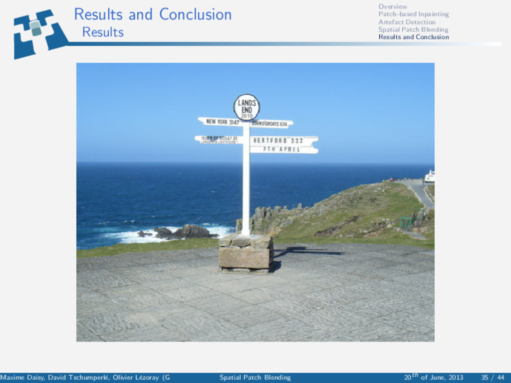
35. Overview Patch-based Inpainting Artefact Detection Spatial Patch Blending Results and Conclusion Results and Conclusion Results Maxime Daisy, David Tschumperl´ e, Olivier L´ ezoray (GREYC) Spatial Patch Blending 20th of June, 2013 35 / 44
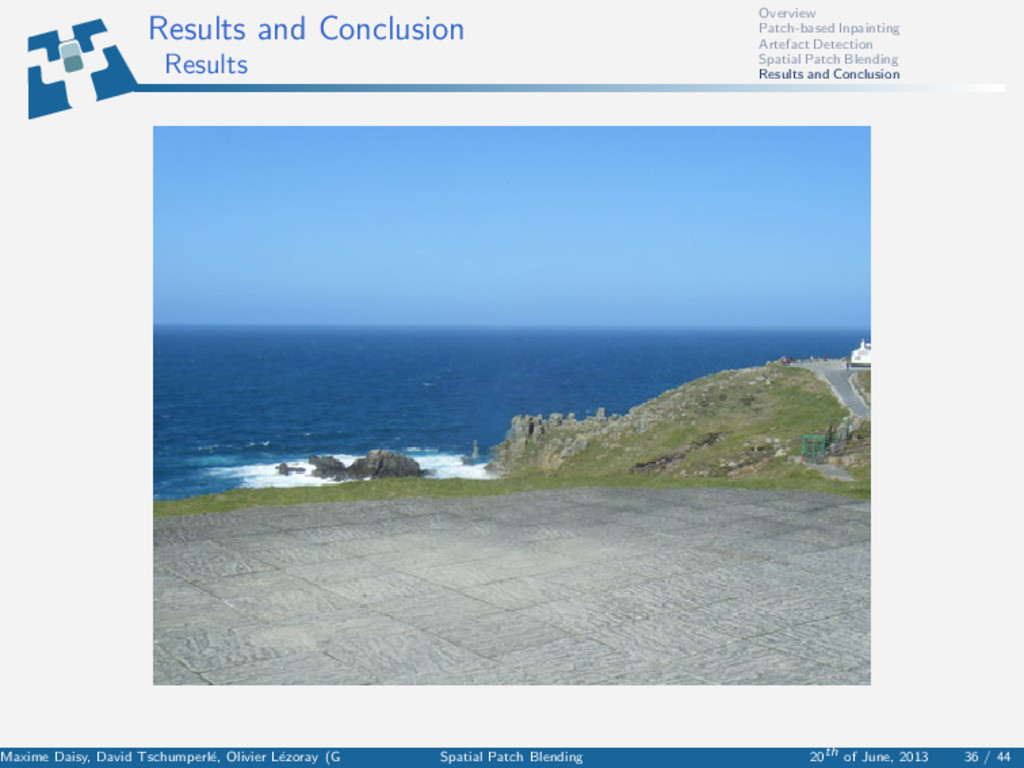
36. Overview Patch-based Inpainting Artefact Detection Spatial Patch Blending Results and Conclusion Results and Conclusion Results Maxime Daisy, David Tschumperl´ e, Olivier L´ ezoray (GREYC) Spatial Patch Blending 20th of June, 2013 36 / 44
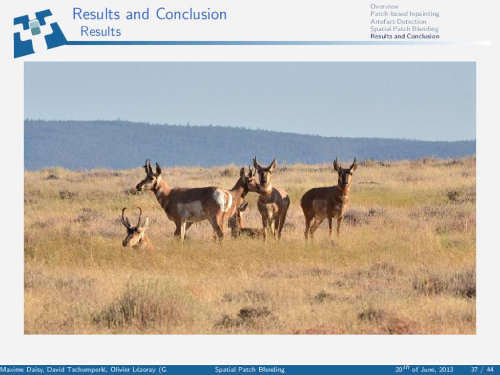
37. Overview Patch-based Inpainting Artefact Detection Spatial Patch Blending Results and Conclusion Results and Conclusion Results Maxime Daisy, David Tschumperl´ e, Olivier L´ ezoray (GREYC) Spatial Patch Blending 20th of June, 2013 37 / 44
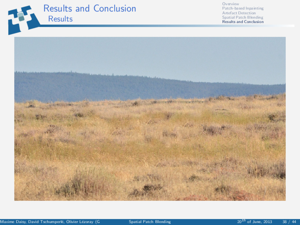
38. Overview Patch-based Inpainting Artefact Detection Spatial Patch Blending Results and Conclusion Results and Conclusion Results Maxime Daisy, David Tschumperl´ e, Olivier L´ ezoray (GREYC) Spatial Patch Blending 20th of June, 2013 38 / 44
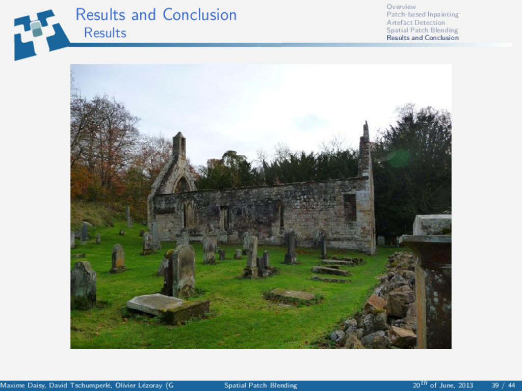
39. Overview Patch-based Inpainting Artefact Detection Spatial Patch Blending Results and Conclusion Results and Conclusion Results Maxime Daisy, David Tschumperl´ e, Olivier L´ ezoray (GREYC) Spatial Patch Blending 20th of June, 2013 39 / 44
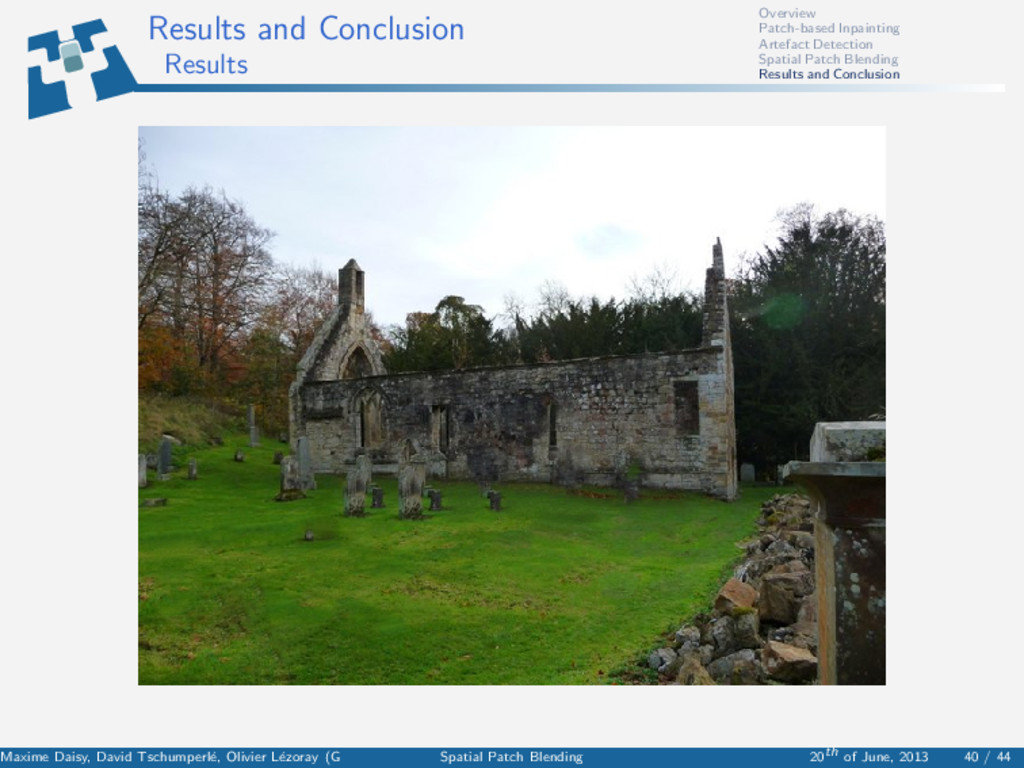
40. Overview Patch-based Inpainting Artefact Detection Spatial Patch Blending Results and Conclusion Results and Conclusion Results Maxime Daisy, David Tschumperl´ e, Olivier L´ ezoray (GREYC) Spatial Patch Blending 20th of June, 2013 40 / 44
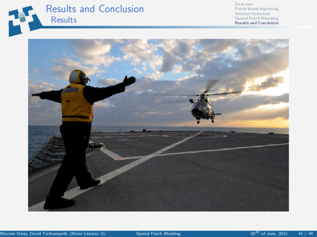
41. Overview Patch-based Inpainting Artefact Detection Spatial Patch Blending Results and Conclusion Results and Conclusion Results Maxime Daisy, David Tschumperl´ e, Olivier L´ ezoray (GREYC) Spatial Patch Blending 20th of June, 2013 41 / 44
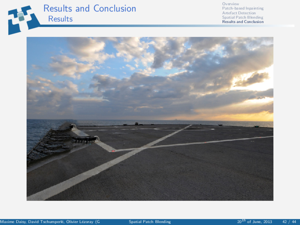
42. Overview Patch-based Inpainting Artefact Detection Spatial Patch Blending Results and Conclusion Results and Conclusion Results Maxime Daisy, David Tschumperl´ e, Olivier L´ ezoray (GREYC) Spatial Patch Blending 20th of June, 2013 42 / 44
43. Overview Patch-based Inpainting Artefact Detection Spatial Patch Blending Results and Conclusion Results and Conclusion Conclusion • Fast seams removal • Lightweight changes to apply to inpainting algorithm. • Few parameters, and easily adjustable. Maxime Daisy, David Tschumperl´ e, Olivier L´ ezoray (GREYC) Spatial Patch Blending 20th of June, 2013 43 / 44
44. Have questions ? Daisy, M., Tschumperl´ e, D., L´ ezoray, O. (2013). Spatial Patch Blending for Artefact Reduction in Pattern-based Inpainting Techniques. CAIP