ICASSP 2017

Transcript

1. 3D colored mesh graph signals multi-layer morphological enhancement Olivier L´ ezoray Normandie Univ, UNICAEN, ENSICAEN, CNRS, GREYC, 14000 Caen, France olivier.lezoray@unicaen.fr https://lezoray.users.greyc.fr
2. 1 Introduction and Motivations 2 Morphological processing of 3D colored graph signals 3 Graph signal representation and morphological processing 4 Multi-layer morphological enhancement 5 Conclusions and perspectives 2 / 35
3. 1 Introduction and Motivations 2 Morphological processing of 3D colored graph signals 3 Graph signal representation and morphological processing 4 Multi-layer morphological enhancement 5 Conclusions and perspectives 3 / 35
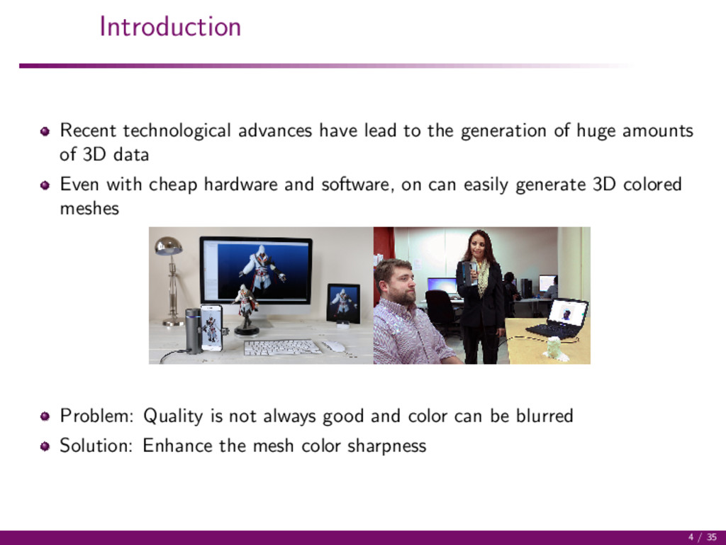
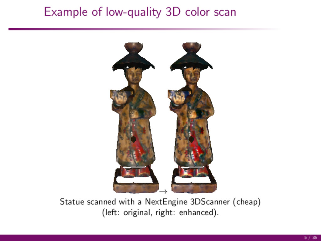
4. Introduction Recent technological advances have lead to the generation of huge amounts of 3D data Even with cheap hardware and software, on can easily generate 3D colored meshes Problem: Quality is not always good and color can be blurred Solution: Enhance the mesh color sharpness 4 / 35
5. Example of low-quality 3D color scan Statue scanned with a NextEngine 3DScanner (cheap) 5 / 35
6. Example of low-quality 3D color scan → Statue scanned with a NextEngine 3DScanner (cheap) (left: original, right: enhanced). 5 / 35
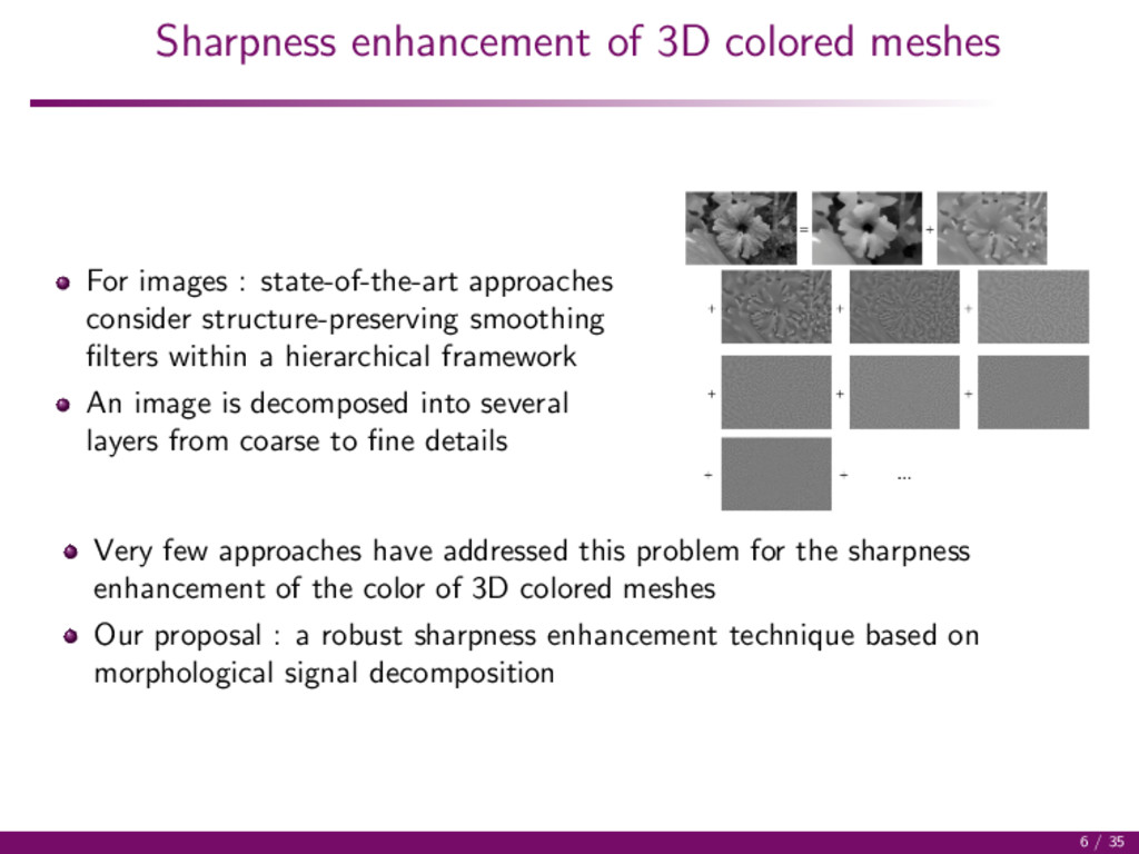
7. Sharpness enhancement of 3D colored meshes For images : state-of-the-art approaches consider structure-preserving smoothing filters within a hierarchical framework An image is decomposed into several layers from coarse to fine details Very few approaches have addressed this problem for the sharpness enhancement of the color of 3D colored meshes Our proposal : a robust sharpness enhancement technique based on morphological signal decomposition 6 / 35
8. 1 Introduction and Motivations 2 Morphological processing of 3D colored graph signals 3 Graph signal representation and morphological processing 4 Multi-layer morphological enhancement 5 Conclusions and perspectives 7 / 35
9. 1 Introduction and Motivations 2 Morphological processing of 3D colored graph signals 3 Graph signal representation and morphological processing 4 Multi-layer morphological enhancement 5 Conclusions and perspectives 8 / 35
10. Graph signals We consider the case of 3D colored signals defined on a domain represented by a graph (a triangulated mesh). A graph G = (V, E) consists in a set V = {v1, . . . , vm} of vertices and a set E ⊂ V × V of edges connecting vertices. A graph signal is a function that associates real-valued vectors to vertices of the graph f : G → T ⊂ Rn. The set T = {v1, · · · , vm} represents all the vectors associated to all vertices of the graph To each vertex vi ∈ G is associated a vector f (vi ) = vi = T [i]. 9 / 35
11. Complete Lattice To process graph signals, we build a new signal representation in the form of an index associated with an ordering of the vectors T of an graph signal. Ordering all the values of the set T can be done with the use of an ordering relation within vectors. This amounts to dispose of a complete lattice (T , ≤) but there is no universal order for vectorial data The framework of h-orderings can be considered for that : construct a surjective mapping h from T to L where L is a complete lattice equipped with the conditional total ordering h : T → L and v → h(v), ∀(vi , vj ) ∈ T × T vi ≤h vj ⇔ h(vi ) ≤ h(vj ) . ≤h will denote such an h-ordering 10 / 35
12. Manifold-based color ordering × Problem : the projection operator h cannot be linear since a distortion of the space is inevitable ! 11 / 35
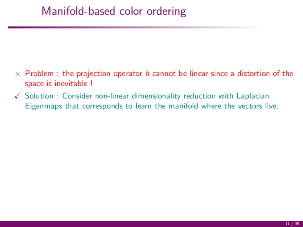
13. Manifold-based color ordering × Problem : the projection operator h cannot be linear since a distortion of the space is inevitable ! Solution : Consider non-linear dimensionality reduction with Laplacian Eigenmaps that corresponds to learn the manifold where the vectors live. 11 / 35
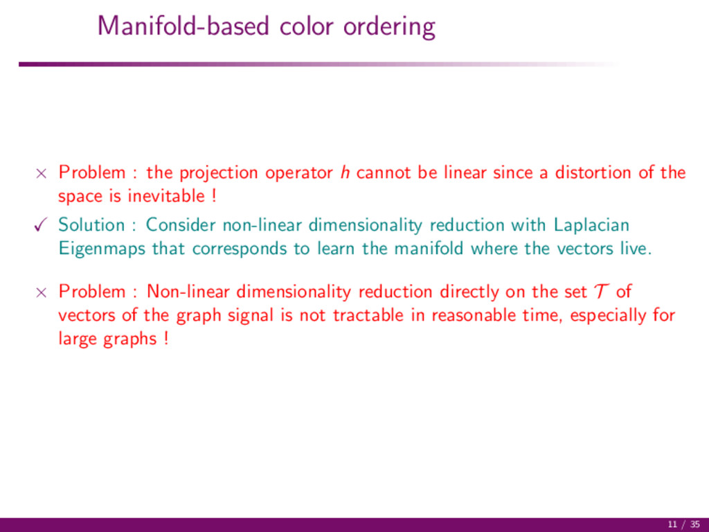
14. Manifold-based color ordering × Problem : the projection operator h cannot be linear since a distortion of the space is inevitable ! Solution : Consider non-linear dimensionality reduction with Laplacian Eigenmaps that corresponds to learn the manifold where the vectors live. × Problem : Non-linear dimensionality reduction directly on the set T of vectors of the graph signal is not tractable in reasonable time, especially for large graphs ! 11 / 35
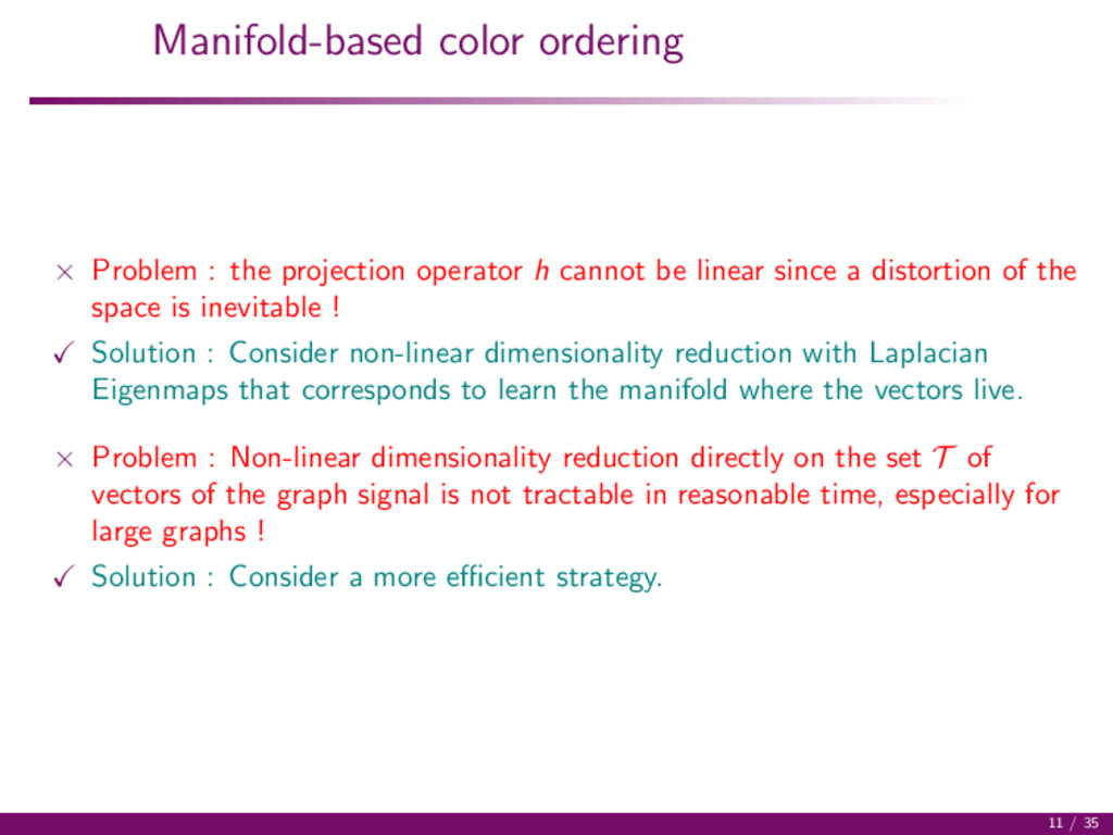
15. Manifold-based color ordering × Problem : the projection operator h cannot be linear since a distortion of the space is inevitable ! Solution : Consider non-linear dimensionality reduction with Laplacian Eigenmaps that corresponds to learn the manifold where the vectors live. × Problem : Non-linear dimensionality reduction directly on the set T of vectors of the graph signal is not tractable in reasonable time, especially for large graphs ! Solution : Consider a more efficient strategy. 11 / 35
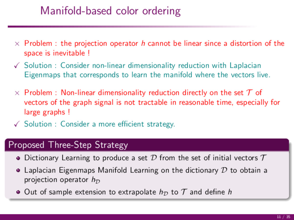
16. Manifold-based color ordering × Problem : the projection operator h cannot be linear since a distortion of the space is inevitable ! Solution : Consider non-linear dimensionality reduction with Laplacian Eigenmaps that corresponds to learn the manifold where the vectors live. × Problem : Non-linear dimensionality reduction directly on the set T of vectors of the graph signal is not tractable in reasonable time, especially for large graphs ! Solution : Consider a more efficient strategy. Proposed Three-Step Strategy Dictionary Learning to produce a set D from the set of initial vectors T Laplacian Eigenmaps Manifold Learning on the dictionary D to obtain a projection operator hD Out of sample extension to extrapolate hD to T and define h 11 / 35
17. Learning the manifold of vectors Step 1: Dictionary Construction Build from T , by Vector Quantization, a dictionary D = {x1 , . . . , xp } with p m Step 2: Manifold Learning on the dictionary Laplacian Eigenmaps Manifold Learning searches Φ such that 1 2 ij Φ(xi ) − Φ(xj ) 2 KD (i, j) = Tr(ΦT LΦ) with ΦT DD Φ = I. Compute the similarity matrix KD between vectors xi ∈ D with KD (i, j) = k(xi , xj ) = exp − xi −xj 2 2 σ2 with σ = max (x i ,x j )∈D xi − xj 2 2 Compute the degree diagonal matrix DD of KD Solution is obtained with the eigen-decomposition of the normalized Laplacian L = I − D− 1 2 D KD D− 1 2 D as L = ΦD ΠD ΦT D with eigenvectors ΦD = [Φ1 D , · · · , Φp D ] and eigenvalues ΠD = diag[λ1, · · · , λp ] 12 / 35
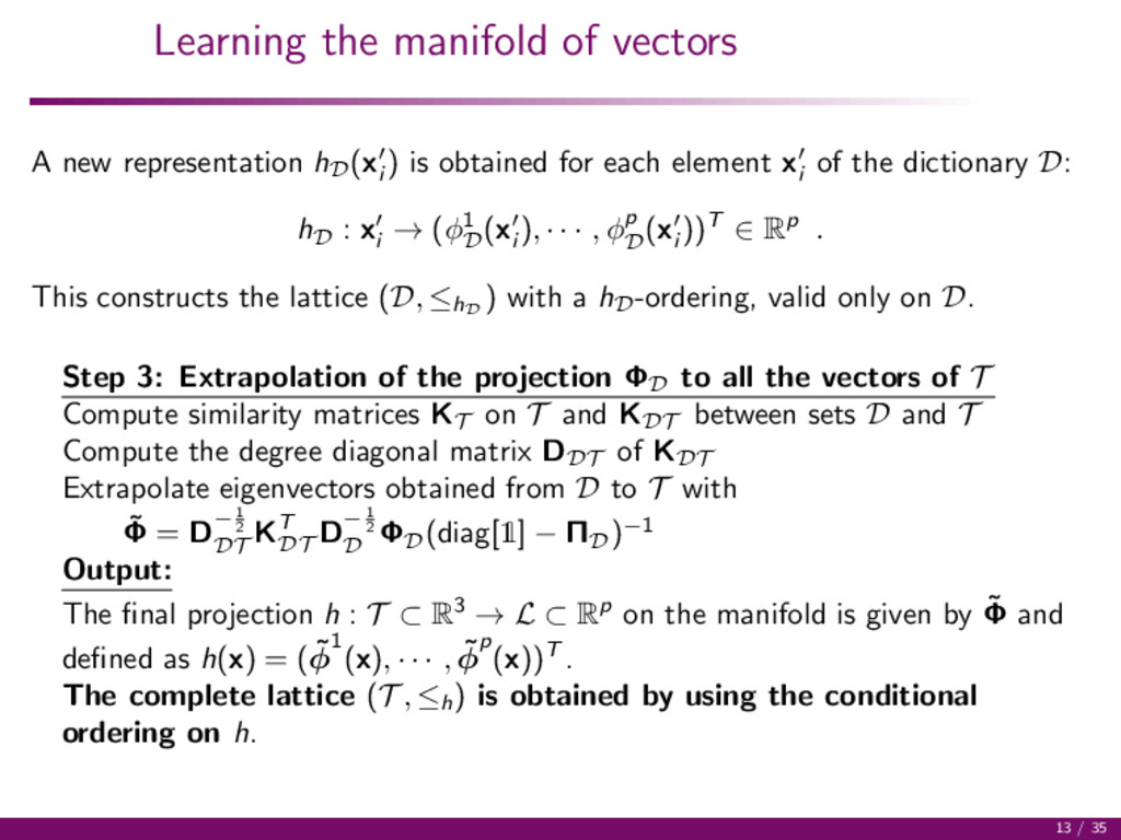
18. Learning the manifold of vectors A new representation hD (xi ) is obtained for each element xi of the dictionary D: hD : xi → (φ1 D (xi ), · · · , φp D (xi ))T ∈ Rp . This constructs the lattice (D, ≤hD ) with a hD -ordering, valid only on D. Step 3: Extrapolation of the projection ΦD to all the vectors of T Compute similarity matrices KT on T and KDT between sets D and T Compute the degree diagonal matrix DDT of KDT Extrapolate eigenvectors obtained from D to T with ˜ Φ = D− 1 2 DT KT DT D− 1 2 D ΦD (diag[1] − ΠD )−1 Output: The final projection h : T ⊂ R3 → L ⊂ Rp on the manifold is given by ˜ Φ and defined as h(x) = ( ˜ φ1 (x), · · · , ˜ φp (x))T . The complete lattice (T , ≤h ) is obtained by using the conditional ordering on h. 13 / 35
19. 1 Introduction and Motivations 2 Morphological processing of 3D colored graph signals 3 Graph signal representation and morphological processing 4 Multi-layer morphological enhancement 5 Conclusions and perspectives 14 / 35
20. 1 Introduction and Motivations 2 Morphological processing of 3D colored graph signals 3 Graph signal representation and morphological processing 4 Multi-layer morphological enhancement 5 Conclusions and perspectives 15 / 35
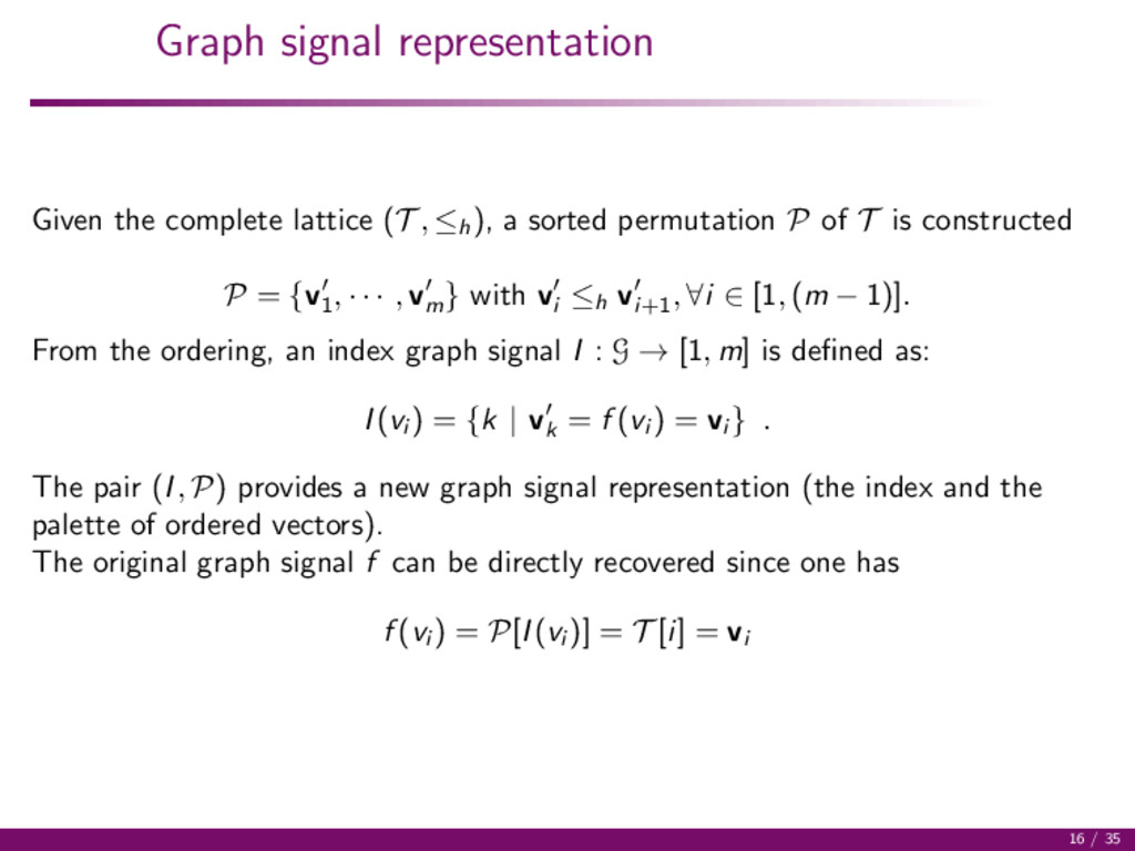
21. Graph signal representation Given the complete lattice (T , ≤h ), a sorted permutation P of T is constructed P = {v1 , · · · , vm } with vi ≤h vi+1 , ∀i ∈ [1, (m − 1)]. From the ordering, an index graph signal I : G → [1, m] is defined as: I(vi ) = {k | vk = f (vi ) = vi } . The pair (I, P) provides a new graph signal representation (the index and the palette of ordered vectors). The original graph signal f can be directly recovered since one has f (vi ) = P[I(vi )] = T [i] = vi 16 / 35
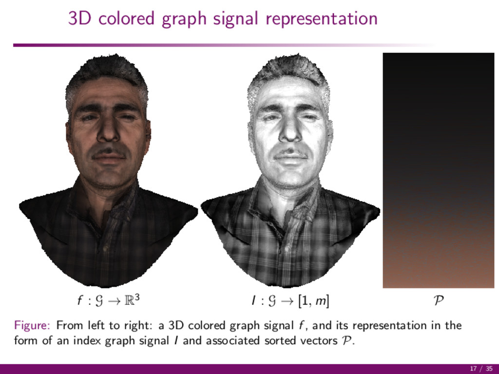
22. 3D colored graph signal representation f : G → R3 I : G → [1, m] P Figure: From left to right: a 3D colored graph signal f , and its representation in the form of an index graph signal I and associated sorted vectors P. 17 / 35
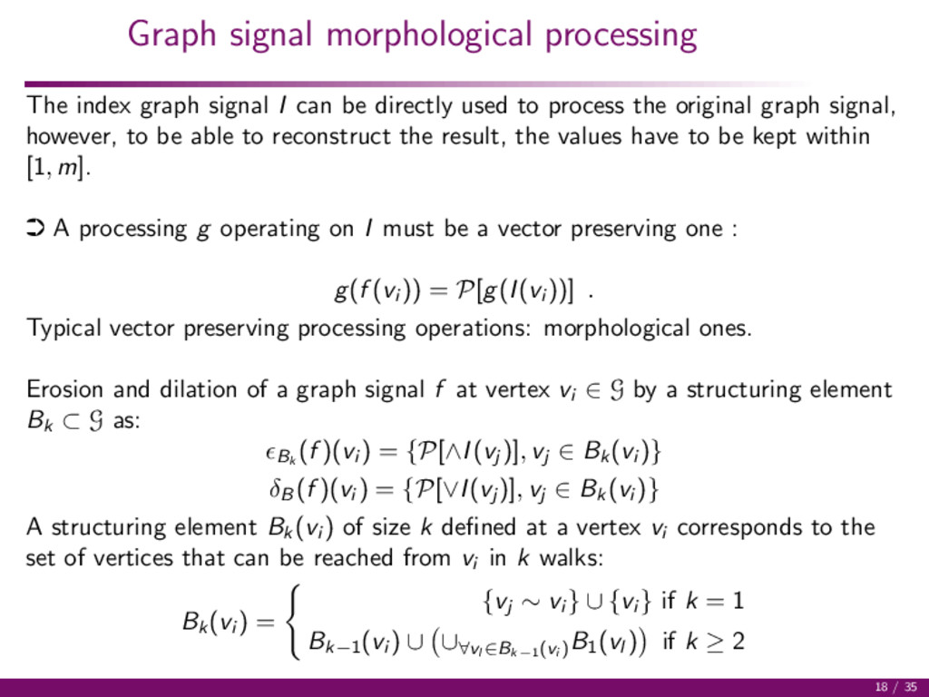
23. Graph signal morphological processing The index graph signal I can be directly used to process the original graph signal, however, to be able to reconstruct the result, the values have to be kept within [1, m]. · A processing g operating on I must be a vector preserving one : g(f (vi )) = P[g(I(vi ))] . Typical vector preserving processing operations: morphological ones. Erosion and dilation of a graph signal f at vertex vi ∈ G by a structuring element Bk ⊂ G as: Bk (f )(vi ) = {P[∧I(vj )], vj ∈ Bk (vi )} δB (f )(vi ) = {P[∨I(vj )], vj ∈ Bk (vi )} A structuring element Bk (vi ) of size k defined at a vertex vi corresponds to the set of vertices that can be reached from vi in k walks: Bk (vi ) = {vj ∼ vi } ∪ {vi } if k = 1 Bk−1 (vi ) ∪ ∪∀vl ∈Bk−1(vi ) B1 (vl ) if k ≥ 2 18 / 35
24. 1 Introduction and Motivations 2 Morphological processing of 3D colored graph signals 3 Graph signal representation and morphological processing 4 Multi-layer morphological enhancement 5 Conclusions and perspectives 19 / 35
25. 1 Introduction and Motivations 2 Morphological processing of 3D colored graph signals 3 Graph signal representation and morphological processing 4 Multi-layer morphological enhancement 5 Conclusions and perspectives 20 / 35
26. Graph signal multi-layer decomposition We propose the following multi-layer morphological decomposition of a graph signal into l layers. The graph signal is decomposed into a base layer and several detail layers, each capturing a given scale of details. d−1 = f , i = 0 while i < l do Compute the graph signal representation at level i − 1: di−1 = (Ii−1, Pi−1 ) Morphological Filtering of di−1 : fi = MFBl−i (di−1 ) Compute the residual (detail layer): di = di−1 − fi Proceed to next layer: i = i + 1 end while 21 / 35
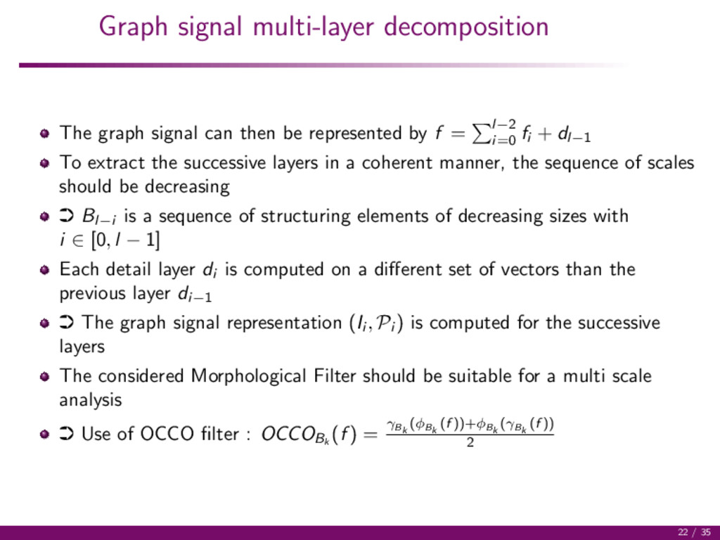
27. Graph signal multi-layer decomposition The graph signal can then be represented by f = l−2 i=0 fi + dl−1 To extract the successive layers in a coherent manner, the sequence of scales should be decreasing · Bl−i is a sequence of structuring elements of decreasing sizes with i ∈ [0, l − 1] Each detail layer di is computed on a different set of vectors than the previous layer di−1 · The graph signal representation (Ii , Pi ) is computed for the successive layers The considered Morphological Filter should be suitable for a multi scale analysis · Use of OCCO filter : OCCOBk (f ) = γBk (φBk (f ))+φBk (γBk (f )) 2 22 / 35
28. Decomposition example Figure: From top to bottom, left to right: an original mesh f , and its decomposition into three layers f0 , f1 , and d1 . 23 / 35
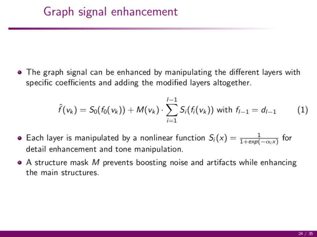
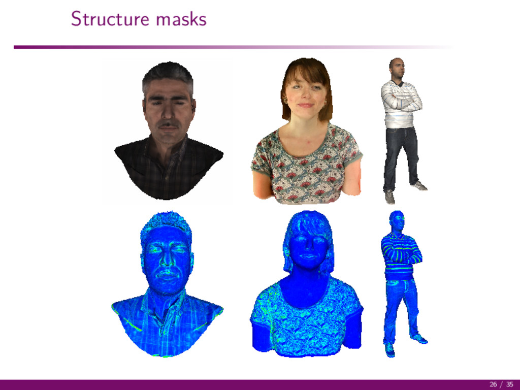
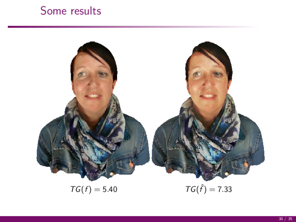
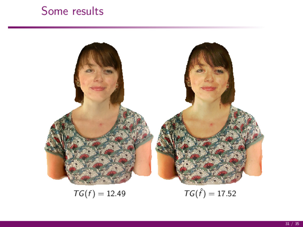
29. Graph signal enhancement The graph signal can be enhanced by manipulating the different layers with specific coefficients and adding the modified layers altogether. ˆ f (vk ) = S0 (f0 (vk )) + M(vk ) · l−1 i=1 Si (fi (vk )) with fl−1 = dl−1 (1) Each layer is manipulated by a nonlinear function Si (x) = 1 1+exp(−αi x) for detail enhancement and tone manipulation. A structure mask M prevents boosting noise and artifacts while enhancing the main structures. 24 / 35
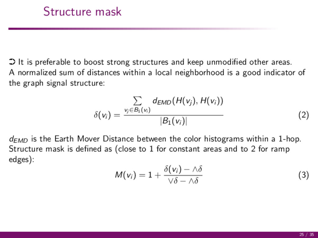
30. Structure mask · It is preferable to boost strong structures and keep unmodified other areas. A normalized sum of distances within a local neighborhood is a good indicator of the graph signal structure: δ(vi ) = vj ∈B1(vi ) dEMD (H(vj ), H(vi )) |B1 (vi )| (2) dEMD is the Earth Mover Distance between the color histograms within a 1-hop. Structure mask is defined as (close to 1 for constant areas and to 2 for ramp edges): M(vi ) = 1 + δ(vi ) − ∧δ ∨δ − ∧δ (3) 25 / 35
31. Structure masks 26 / 35
32. Some results TG(f ) = 3.86 TG(ˆ f ) = 5.40 27 / 35
33. Some results 28 / 35
34. Some results 29 / 35
35. Some results TG(f ) = 5.40 TG(ˆ f ) = 7.33 30 / 35
36. Some results TG(f ) = 12.49 TG(ˆ f ) = 17.52 31 / 35
37. 1 Introduction and Motivations 2 Morphological processing of 3D colored graph signals 3 Graph signal representation and morphological processing 4 Multi-layer morphological enhancement 5 Conclusions and perspectives 32 / 35
38. 1 Introduction and Motivations 2 Morphological processing of 3D colored graph signals 3 Graph signal representation and morphological processing 4 Multi-layer morphological enhancement 5 Conclusions and perspectives 33 / 35
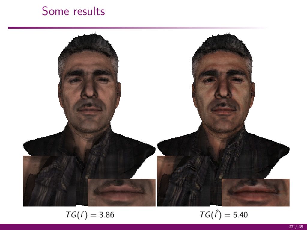
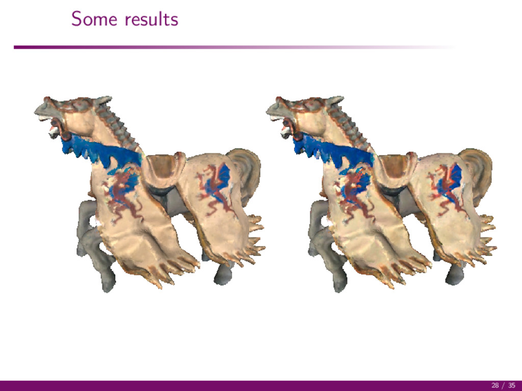
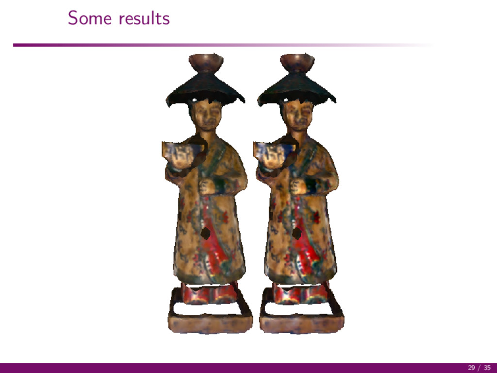
39. Conclusions and perspectives We have proposed: A representation of 3D colored graph signals in the form of a graph index and palette A morphological multi-layer decomposition of graph signals A layer manipulation approach for graph signal enhancement ·The approach can enhance the sharpness of 3D colored meshes 34 / 35
40. The end Publications available at : https://lezoray.users.greyc.fr Work funded under ANR-14-CE27-0001 GRAPHSIP and from the European Union FEDER/FSE 2014/2020 (GRAPHSIP project) 35 / 35