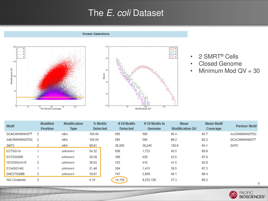
Base Modification Hands On

Transcript

1. Investigating Base Modification Data Outside of SMRT® Portal
2. Learning Objectives 2 Bioinformaticians • Interested in delving into the base-modification workflow output, particularly with bacterial data sets • Requiring information on experimental design for DNA Base Modification Projects After the training, you will be able to • Understand the features available in SMRT® Analysis v2.0.1+ that assist in detection of modified bases • Be familiar with tools available to assist in deep dive analyses • Understand the potential benefits of a deep dive analysis • SMRT® Technology • PacBio® System Workflow • Experimental Design for De Novo Assembly
3. Base Modification Workflow Output Several output files are generated by the new analysis protocol • modifications.csv file: – Comma-separated values (CSV) file with statistical analysis of each position in the reference – Intended to allow additional follow-up analysis for every genomic position • modifications.gff file: – General Features Format (GFF) file – Used for motif analysis and modification visualization in SMRT® View – Includes sequence contexts for sites of putative modification − positions where the inter-pulse duration (IPD) is significantly different from the expected background − p-values of 0.01 or less (QV = 20) – SMRT View has been enhanced to take advantage of specific features in this GFF • motif_summary.csv file: – Comma-separated vales (CSV) file with the information displayed in the Motifs report • Files can be downloaded from the DATA section of the SMRT Portal Job Details Page 3
4. Further Examining Base-Modification Results Using R • We have written a number of functions to facilitate more in-depth or custom analysis in R: – Do more nuanced, custom filtering of hits by score and coverage – Annotate any motif of interest in both the gff/contexts and the genome reference – Plot the score vs. coverage distribution by base – Examine the distribution of score, coverage, IPD Ratio or other factors for any motif of interest, both modified or unmodified – Visualize your results using circos • Example data and R functions can be found online: – https://github.com/PacificBiosciences/Bioinformatics- Training/tree/master/basemods – http://pacb.com/bmd/ (basemod data sets at PacBio) – https://github.com/PacificBiosciences/R-kinetics (github R Kinetics package) 4
5. The E. coli Dataset 5 • 2 SMRT® Cells • Closed Genome • Minimum Mod QV = 30
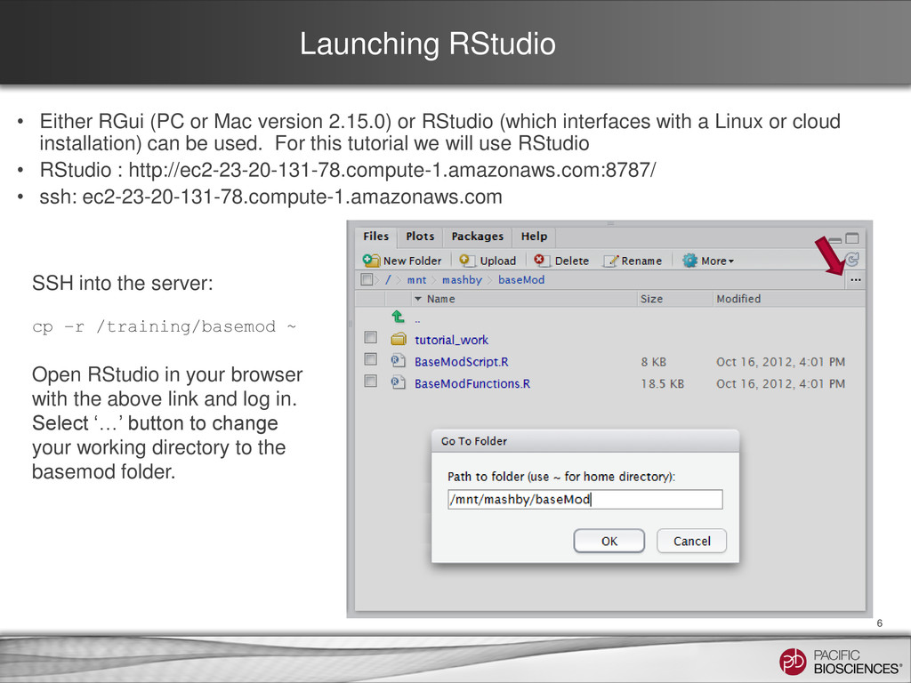
6. Launching RStudio • Either RGui (PC or Mac version 2.15.0) or RStudio (which interfaces with a Linux or cloud installation) can be used. For this tutorial we will use RStudio • RStudio : http://ec2-23-20-131-78.compute-1.amazonaws.com:8787/ • ssh: ec2-23-20-131-78.compute-1.amazonaws.com 6 SSH into the server: cp –r /training/basemod ~ Open RStudio in your browser with the above link and log in. Select ‘…’ button to change your working directory to the basemod folder.
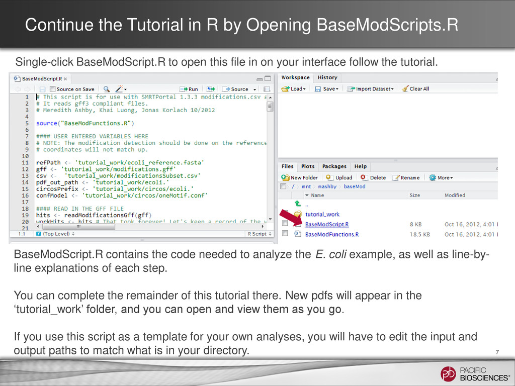
7. Continue the Tutorial in R by Opening BaseModScripts.R Single-click BaseModScript.R to open this file in on your interface follow the tutorial. 7 BaseModScript.R contains the code needed to analyze the E. coli example, as well as line-by- line explanations of each step. You can complete the remainder of this tutorial there. New pdfs will appear in the ‘tutorial_work’ folder, and you can open and view them as you go. If you use this script as a template for your own analyses, you will have to edit the input and output paths to match what is in your directory.
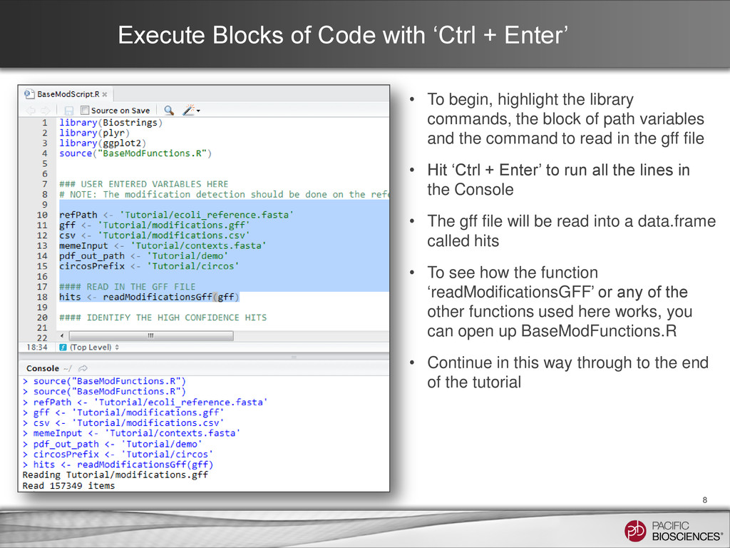
8. Execute Blocks of Code with ‘Ctrl + Enter’ • To begin, highlight the library commands, the block of path variables and the command to read in the gff file • Hit ‘Ctrl + Enter’ to run all the lines in the Console • The gff file will be read into a data.frame called hits • To see how the function ‘readModificationsGFF’ or any of the other functions used here works, you can open up BaseModFunctions.R • Continue in this way through to the end of the tutorial 8
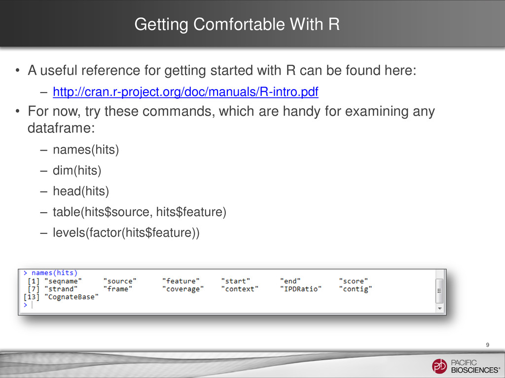
9. Getting Comfortable With R • A useful reference for getting started with R can be found here: – http://cran.r-project.org/doc/manuals/R-intro.pdf • For now, try these commands, which are handy for examining any dataframe: – names(hits) – dim(hits) – head(hits) – table(hits$source, hits$feature) – levels(factor(hits$feature)) 9
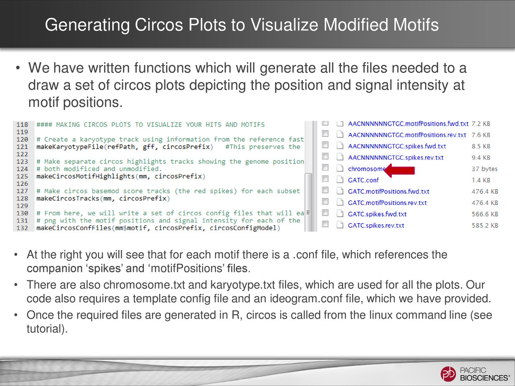
10. Generating Circos Plots to Visualize Modified Motifs • We have written functions which will generate all the files needed to a draw a set of circos plots depicting the position and signal intensity at motif positions. • At the right you will see that for each motif there is a .conf file, which references the companion ‘spikes’ and ‘motifPositions’ files. • There are also chromosome.txt and karyotype.txt files, which are used for all the plots. Our code also requires a template config file and an ideogram.conf file, which we have provided. • Once the required files are generated in R, circos is called from the linux command line (see tutorial).
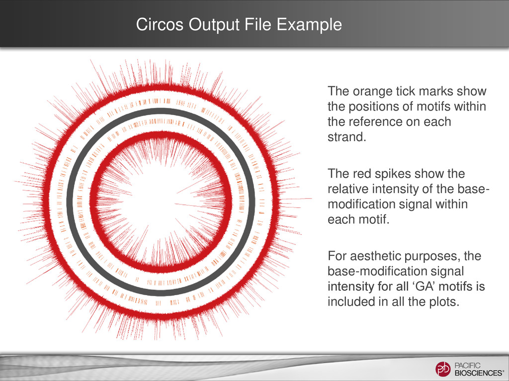
11. Circos Output File Example The orange tick marks show the positions of motifs within the reference on each strand. The red spikes show the relative intensity of the base- modification signal within each motif. For aesthetic purposes, the base-modification signal intensity for all ‘GA’ motifs is included in all the plots.
12. Summary of Key Points • SMRT® Sequencing provides a path to distinguishing numerous different modifications • There are R and Python tools available to help with in-depth examination of base modification data. 12
13. Where to Find Additional Information • http://pacb.com/applications/base_modification/ (PacBio’s basemod resources) • http://svitsrv25.epfl.ch/R-doc/doc/html/search/SearchEngine.html (R search engine) • http://docs.ggplot2.org/current/ (ggplot reference) • http://tools.neb.com/~vincze/genomes/ (REBASE) 13
14. Pacific Biosciences, the Pacific Biosciences logo, PacBio, SMRT, and SMRTbell are trademarks of Pacific Biosciences in the United States and/or other countries. All other trademarks are the sole property of their respective owners.