Machine Learning Models Health-Tech

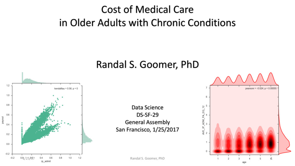
This presentation was made at General Assembly in San Francisco, on January 25, 2017.
It presents newest 'Machine Learning" models in Python.
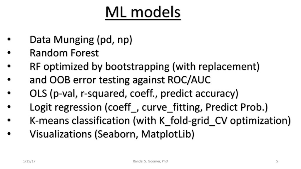
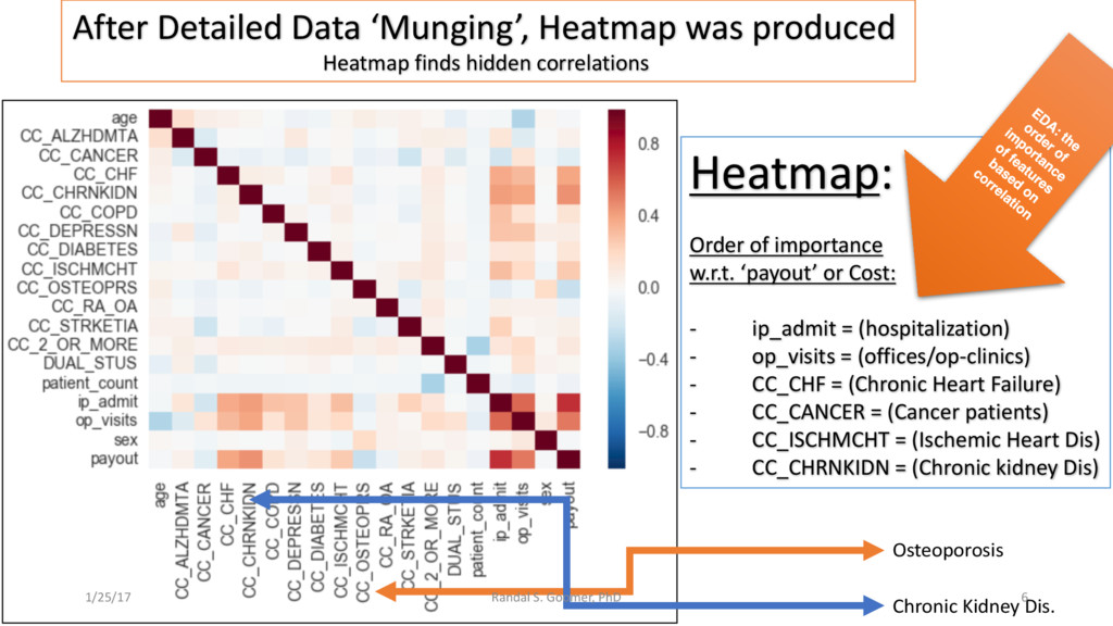
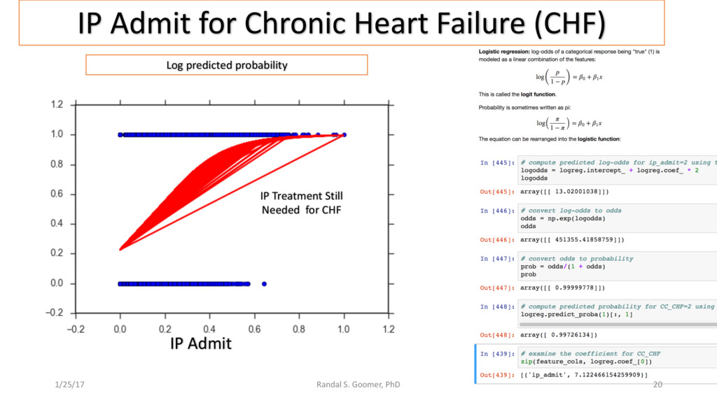
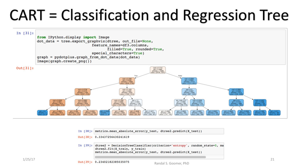
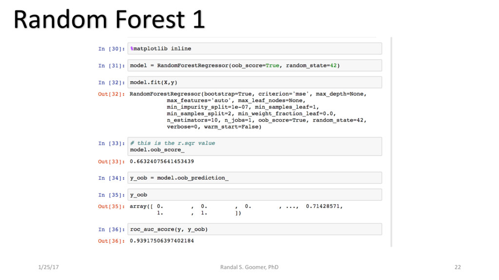
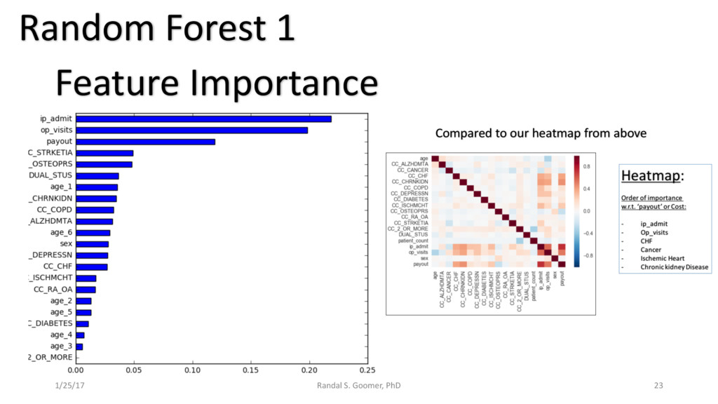
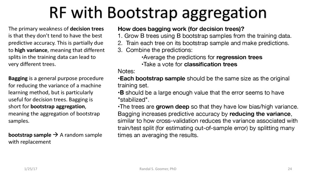
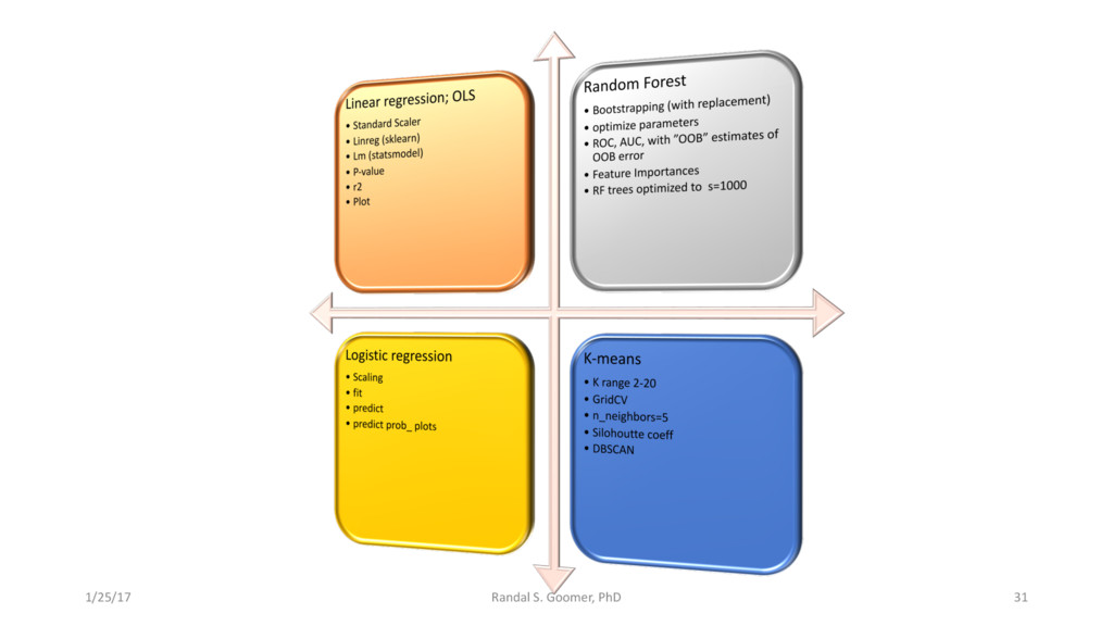
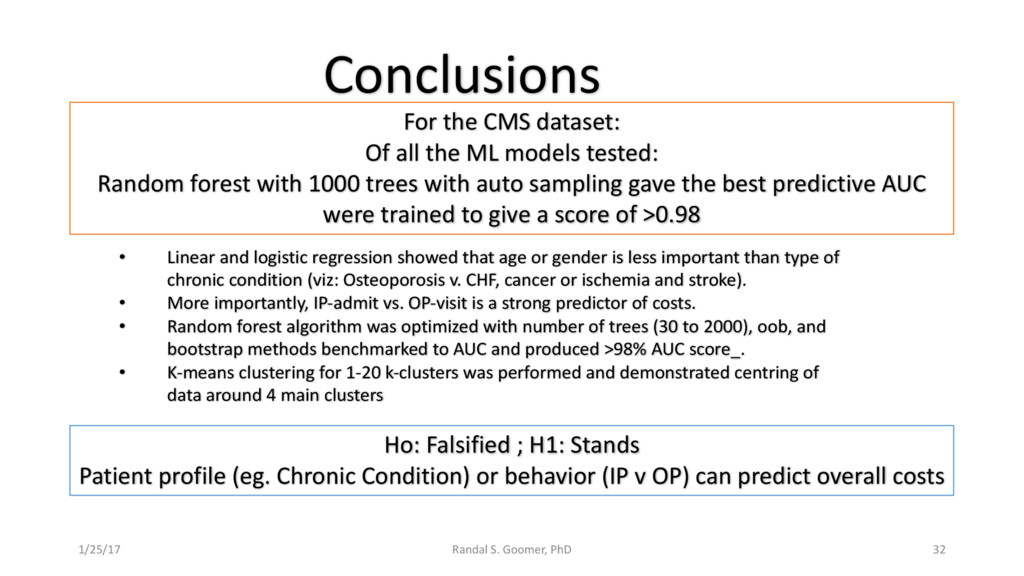
Models used include: 'Random Forest' classification and prediction : bootstrapping optimized with ROC/AUC .Decision Tree algorithm for Health-Tech BI. Advanced Feature selection, Feature scaling and Logistic regression predictions.

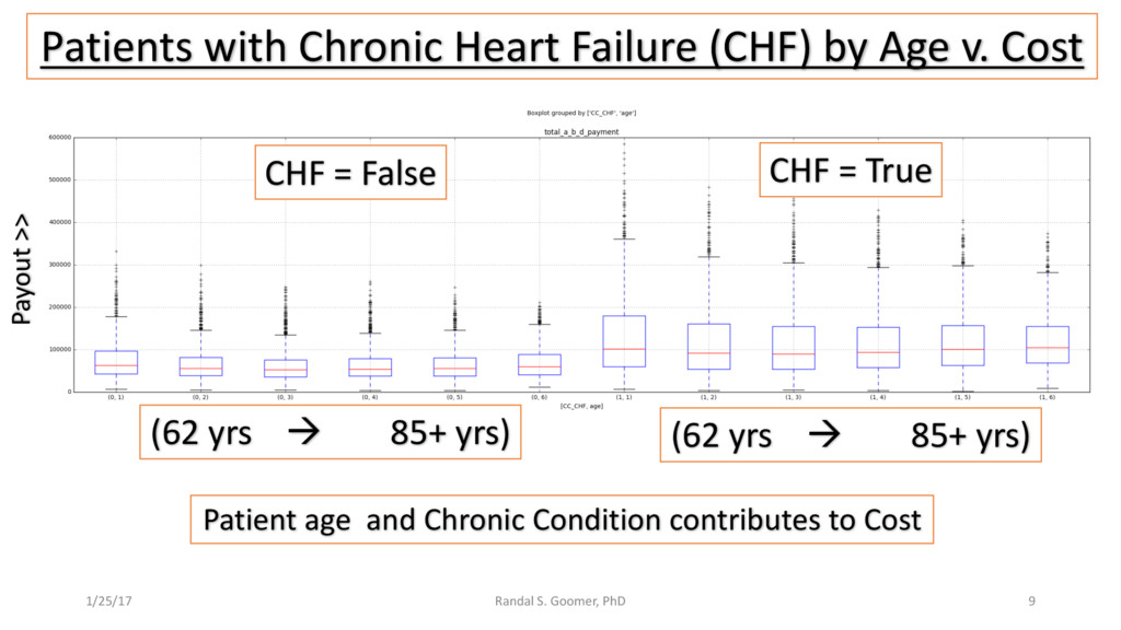
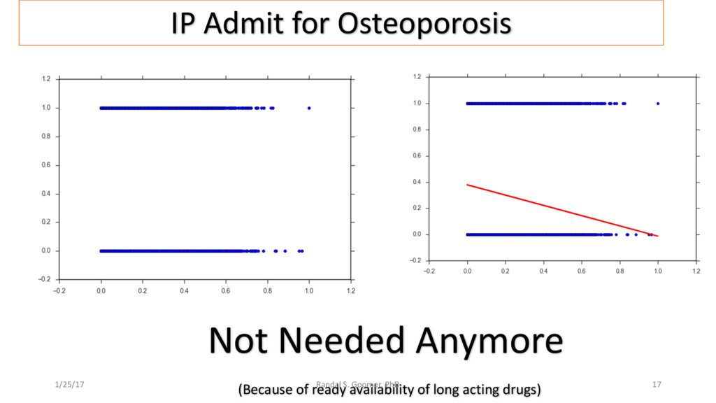
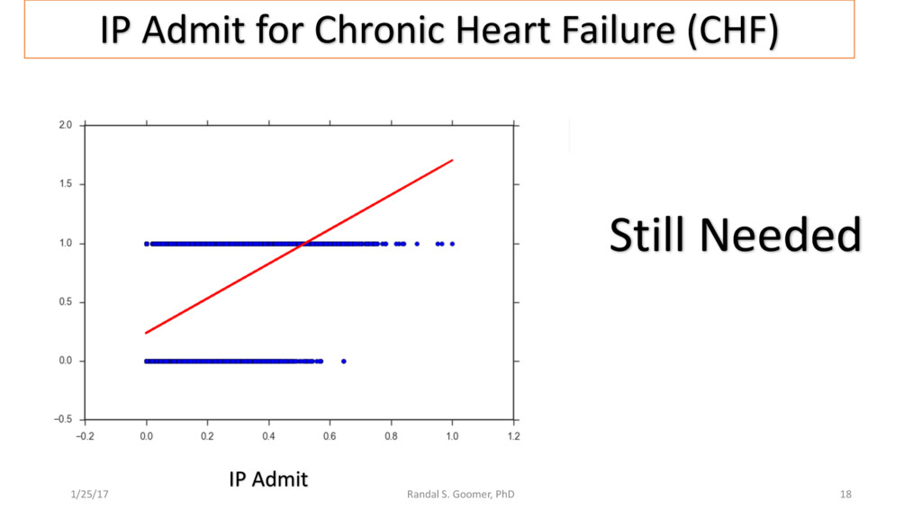
Examples include Chronic Heart Disease v. osteoporosis.
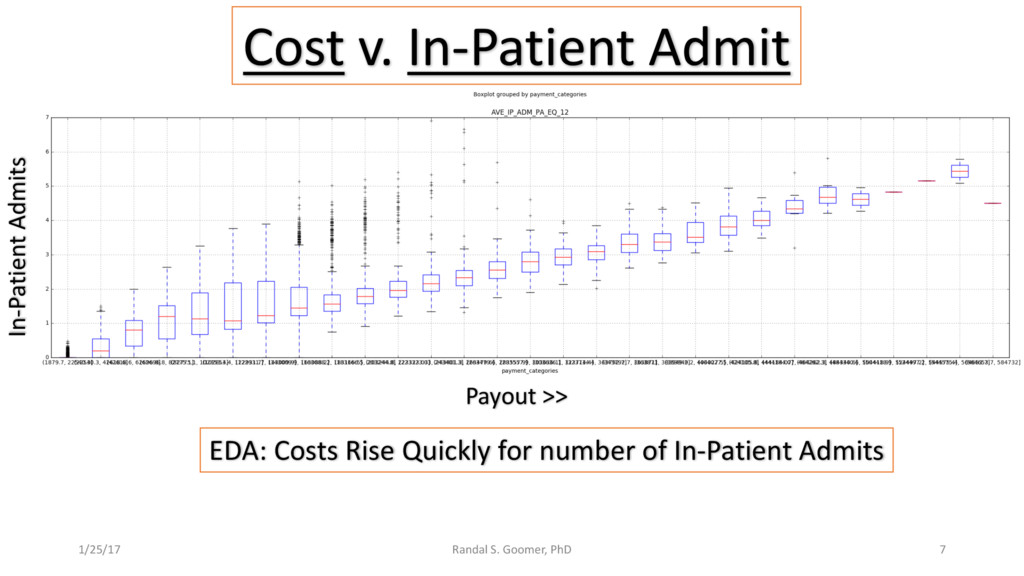
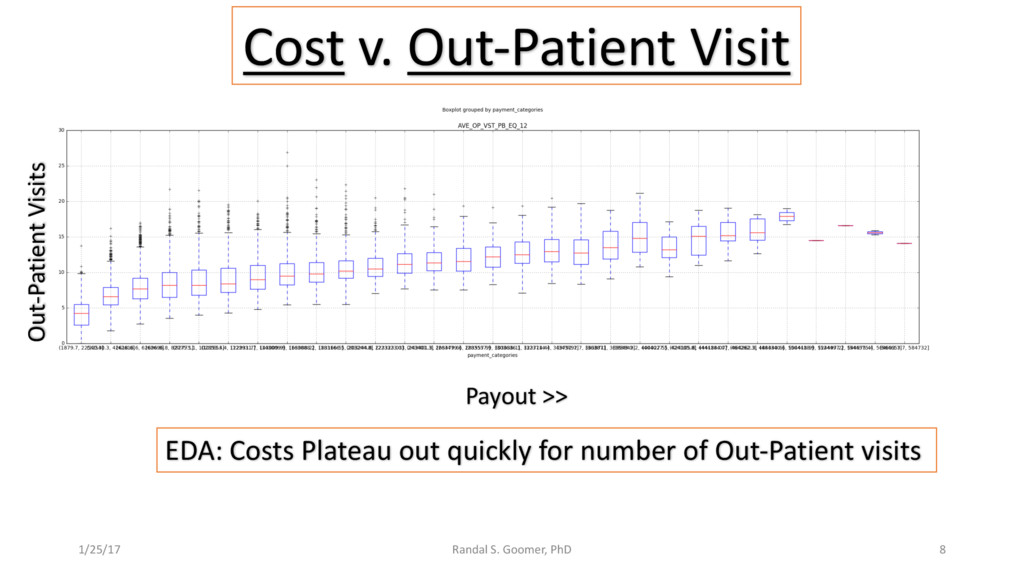
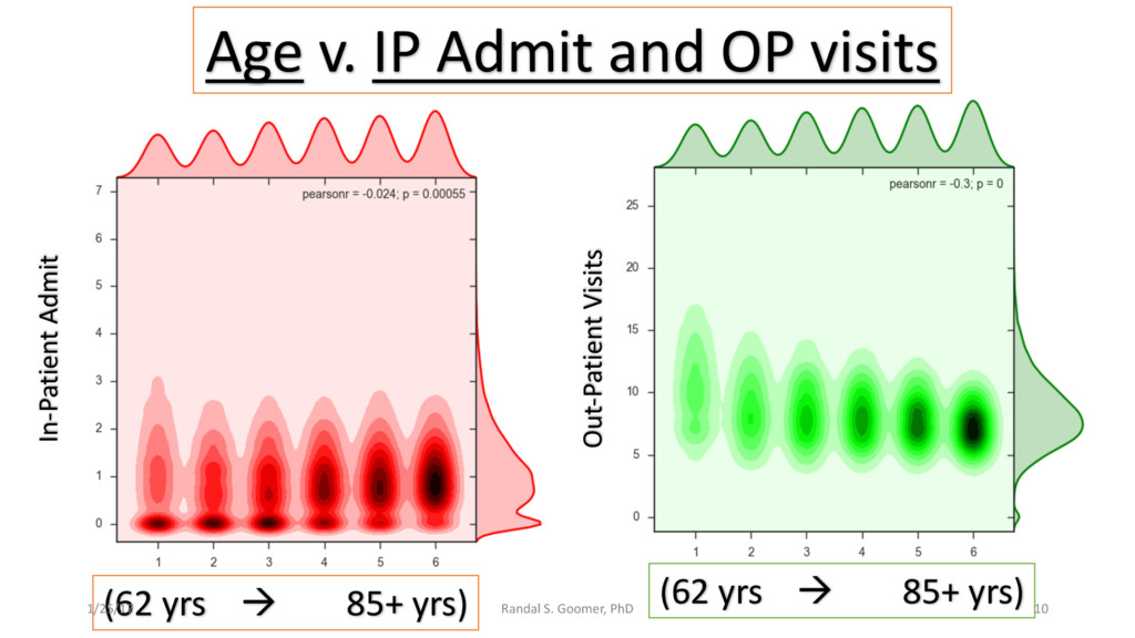
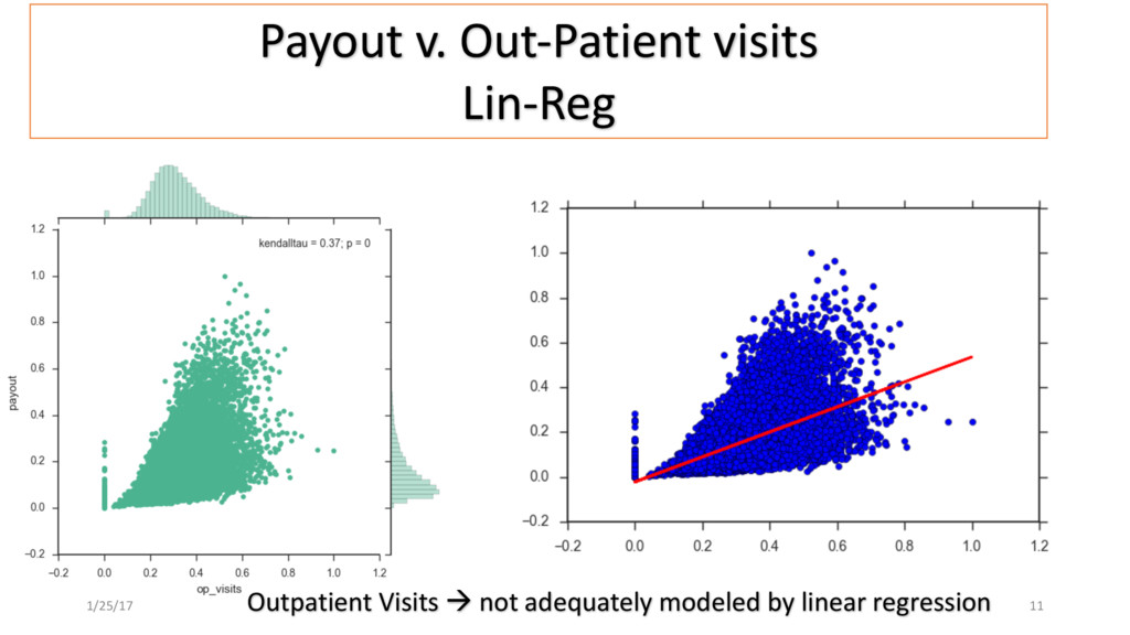
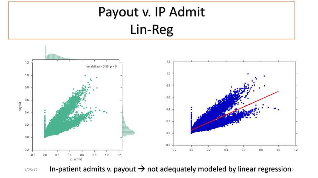
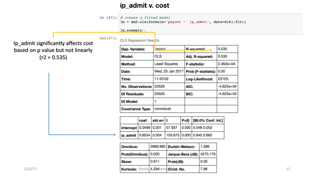
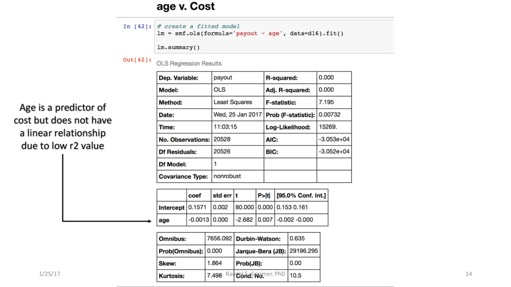
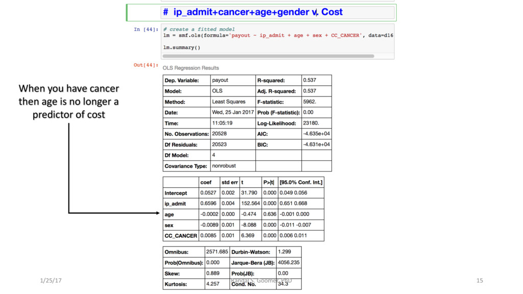
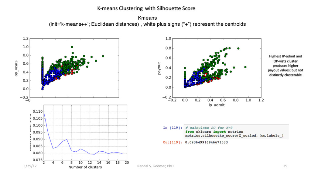
Patient use of in-Patient admits vs. out-patient services as cost minimizer, etc..

Transcript

1. Cost of Medical Care in Older Adults with Chronic Conditions Randal S. Goomer, PhD Data Science DS-SF-29 General Assembly San Francisco, 1/25/2017 Randal S. Goomer, PhD 1/25/17 1
2. DataSet Medicare 2010 Patient records Expunged of all personal or identifiable information (33M patient profiles) Provided by CMS As: 2010 Chronic Conditions PUF (2010 CMS CC PUF) Patient Age Categories: 1 – 6 1. 62-64 2. 65-69 3. 70-74 4. 75-79 5. 80-85 6. 85---- Therapy Behavior: • Number of Out- Patient Visits • Number of In- Patient admits • Medicare Part A, B, C, D, E payments Chronic Conditions à CC • Alzhiemers • Cancer • CHF • Diabetes • ChrKidneyDisease • Stroke • Osteoporosis • Depression • COPD • Ischemic Heart Condition • Stroke • Arthritis Patient Gender Cost (Payouts by Medicare) Randal S. Goomer, PhD 1/25/17 2
3. Dataset Includes a 4-page Dictionary of Terms (Sample: page 1 of 4) Randal S. Goomer, PhD 1/25/17 3
4. Can we predict costs based on patient profile or behavior? BI Questions • Does the type of chronic conditions (CC) impact Costs? • Does age or gender impact cost? • Does patient behavior such as accessing OP facilities vs. IP admits influence costs? • Which behavior costs more of less? • Which CC cost more or less? Ho: <<we cannot predict cost from patient profile and behavior>> H1: <<Patient profile and behavior can predict cost>> Randal S. Goomer, PhD 1/25/17 4
5. ML models • Data Munging (pd, np) • Random Forest • RF optimized by bootstrapping (with replacement) • and OOB error testing against ROC/AUC • OLS (p-val, r-squared, coeff., predict accuracy) • Logit regression (coeff_, curve_fitting, Predict Prob.) • K-means classification (with K_fold-grid_CV optimization) • Visualizations (Seaborn, MatplotLib) Randal S. Goomer, PhD 1/25/17 5
6. Heatmap: Order of importance w.r.t. ‘payout’ or Cost: - ip_admit = (hospitalization) - op_visits = (offices/op-clinics) - CC_CHF = (Chronic Heart Failure) - CC_CANCER = (Cancer patients) - CC_ISCHMCHT = (Ischemic Heart Dis) - CC_CHRNKIDN = (Chronic kidney Dis) After Detailed Data ‘Munging’, Heatmap was produced Heatmap finds hidden correlations Chronic Kidney Dis. Osteoporosis Randal S. Goomer, PhD 1/25/17 6
7. Cost v. In-Patient Admit EDA: Costs Rise Quickly for number of In-Patient Admits Payout >> In-Patient Admits Randal S. Goomer, PhD 1/25/17 7
8. EDA: Costs Plateau out quickly for number of Out-Patient visits Out-Patient Visits Payout >> Cost v. Out-Patient Visit Randal S. Goomer, PhD 1/25/17 8
9. Patients with Chronic Heart Failure (CHF) by Age v. Cost Patient age and Chronic Condition contributes to Cost Payout >> (62 yrs à 85+ yrs) (62 yrs à 85+ yrs) CHF = True CHF = False Randal S. Goomer, PhD 1/25/17 9
10. Age v. IP Admit and OP visits In-Patient Admit In-Patient Admits Out-Patient Visits (62 yrs à 85+ yrs) (62 yrs à 85+ yrs) Randal S. Goomer, PhD 1/25/17 10
11. Payout v. Out-Patient visits Lin-Reg Outpatient Visits à not adequately modeled by linear regression 1/25/17 11
12. Payout v. IP Admit Lin-Reg 1/25/17 12 In-patient admits v. payout à not adequately modeled by linear regression
13. Ip_admit significantly affects cost based on p value but not linearly (r2 = 0.535) Randal S. Goomer, PhD 1/25/17 13
14. Age is a predictor of cost but does not have a linear relationship due to low r2 value Randal S. Goomer, PhD 1/25/17 14
15. When you have cancer then age is no longer a predictor of cost Randal S. Goomer, PhD 1/25/17 15
16. Randal S. Goomer, PhD 1/25/17 16
17. IP Admit for Osteoporosis Not Needed Anymore (Because of ready availability of long acting drugs) Randal S. Goomer, PhD 1/25/17 17
18. IP Admit for Chronic Heart Failure (CHF) IP Admit No Need Still Needed Randal S. Goomer, PhD 1/25/17 18
19. 1/25/17 Randal S. Goomer, PhD 19 Logit Regression
20. IP Admit for Chronic Heart Failure (CHF) Log predicted probability Randal S. Goomer, PhD 1/25/17 20 IP Admit IP Treatment Still Needed for CHF
21. CART = Classification and Regression Tree Randal S. Goomer, PhD 1/25/17 21
22. Random Forest 1 Randal S. Goomer, PhD 1/25/17 22
23. Random Forest 1 Feature Importance Compared to our heatmap from above Randal S. Goomer, PhD 1/25/17 23
24. 1/25/17 Randal S. Goomer, PhD 24 How does bagging work (for decision trees)? 1. Grow B trees using B bootstrap samples from the training data. 2. Train each tree on its bootstrap sample and make predictions. 3. Combine the predictions: •Average the predictions for regression trees •Take a vote for classification trees Notes: •Each bootstrap sample should be the same size as the original training set. •B should be a large enough value that the error seems to have "stabilized". •The trees are grown deep so that they have low bias/high variance. Bagging increases predictive accuracy by reducing the variance, similar to how cross-validation reduces the variance associated with train/test split (for estimating out-of-sample error) by splitting many times an averaging the results. RF with Bootstrap aggregation The primary weakness of decision trees is that they don't tend to have the best predictive accuracy. This is partially due to high variance, meaning that different splits in the training data can lead to very different trees. Bagging is a general purpose procedure for reducing the variance of a machine learning method, but is particularly useful for decision trees. Bagging is short for bootstrap aggregation, meaning the aggregation of bootstrap samples. bootstrap sample à A random sample with replacement
25. Random Forest: Trained n_estimators using bootstrap from 30 to 2,000 Trees using AUC as output; Optimized at 1,000 trees Randal S. Goomer, PhD 1/25/17 25
26. #### the above shows stats when using all features (auto and none), sqrt of features numbers (100 features == 10 used), 90%, or 20%. Random Forest: optimized max-features options, using bootstrap from using AUC as output; ‘auto’, sqrt, log2, 0.9, 0.2 used. Randal S. Goomer, PhD 1/25/17 26
27. Random Forest: optimized min-sample option, using AUC as output. Randal S. Goomer, PhD 1/25/17 27
28. 1/25/17 Randal S. Goomer, PhD 28 K-means clustering to identify cluster behavior Clusters = 1 to 20 Data partitioning into observations of the n- by-p data matrix X into k=4 clusters, returning n-by-1 vector containing cluster indices of each observation. Rows of X corresponded to points and columns corresponded to variables. Separations as squared Euclidean distance measure and the k-means++ algorithm for cluster center initialization
29. K-means Clustering with Silhouette Score Kmeans (init='k-means++’; Euclidean distances) , white plus signs (“+”) represent the centroids Randal S. Goomer, PhD 1/25/17 29 Highest IP-admit and OP-vists cluster produces higher payout values; but not distinctly clusterable
30. K-means Clusters with grid_cv Randal S. Goomer, PhD 1/25/17 30
31. Randal S. Goomer, PhD 1/25/17 31
32. 1/25/17 Randal S. Goomer, PhD 32 Conclusions Ho: Falsified ; H1: Stands Patient profile (eg. Chronic Condition) or behavior (IP v OP) can predict overall costs • Linear and logistic regression showed that age or gender is less important than type of chronic condition (viz: Osteoporosis v. CHF, cancer or ischemia and stroke). • More importantly, IP-admit vs. OP-visit is a strong predictor of costs. • Random forest algorithm was optimized with number of trees (30 to 2000), oob, and bootstrap methods benchmarked to AUC and produced >98% AUC score_. • K-means clustering for 1-20 k-clusters was performed and demonstrated centring of data around 4 main clusters For the CMS dataset: Of all the ML models tested: Random forest with 1000 trees with auto sampling gave the best predictive AUC were trained to give a score of >0.98