A Tale of Two Models: "Traditional" Machine Learning vs Deep Learning

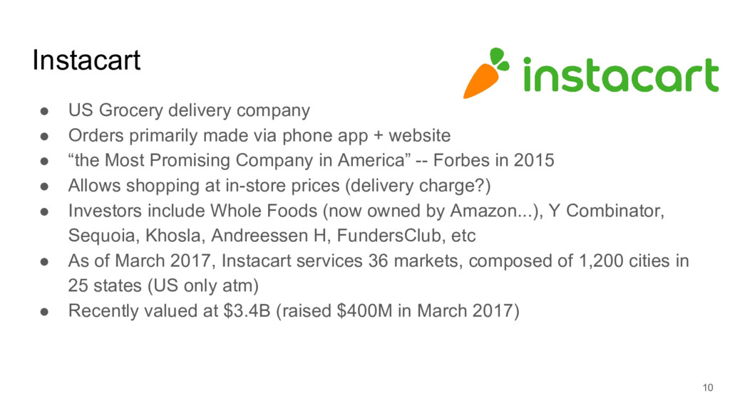
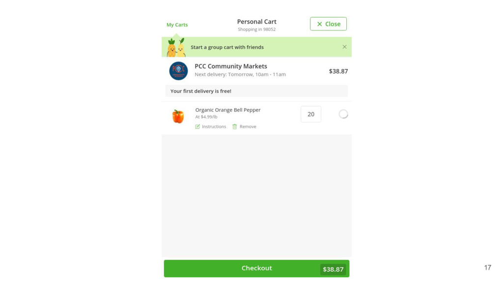
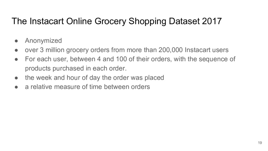
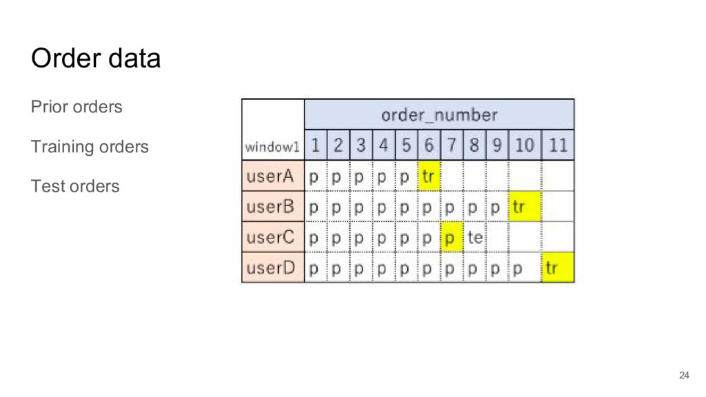
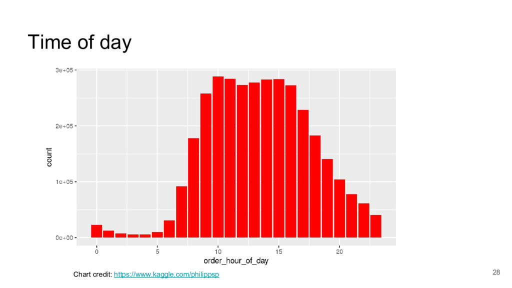
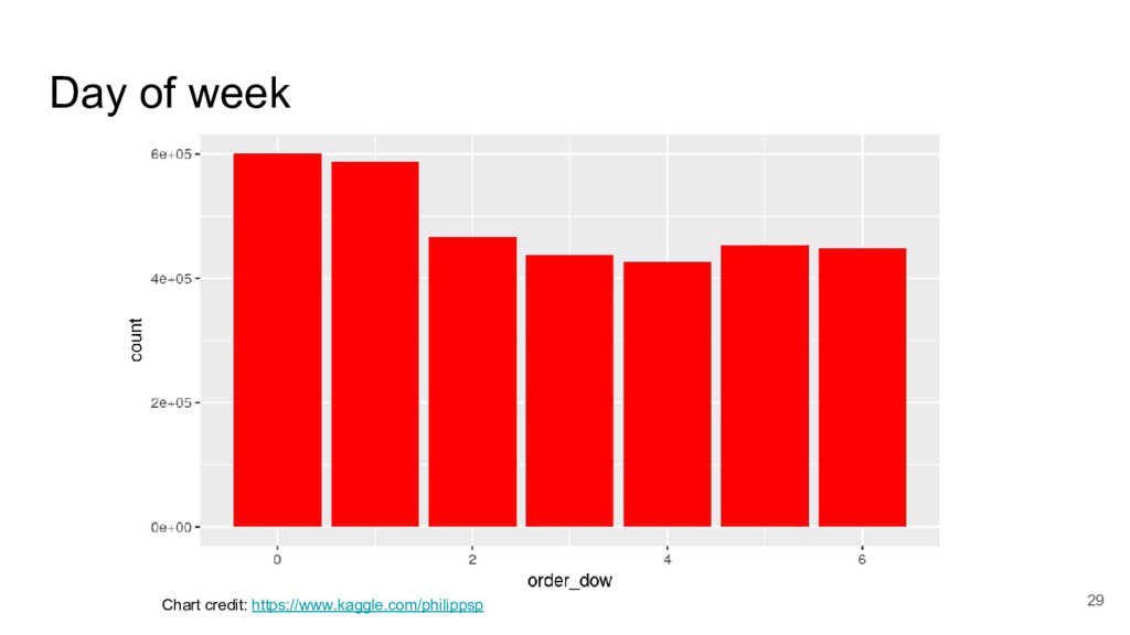
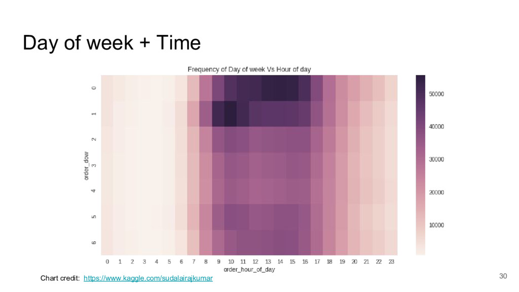
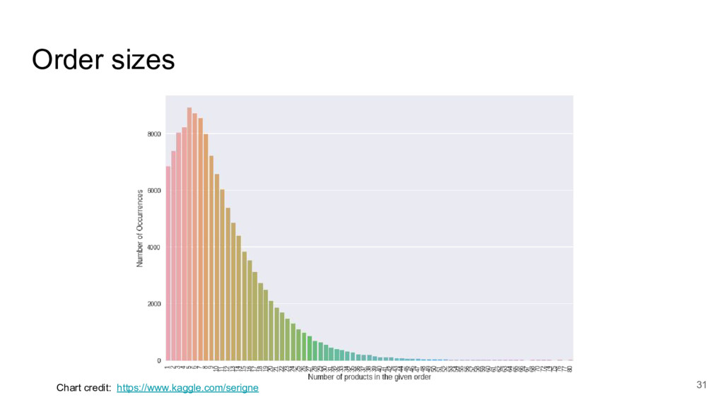
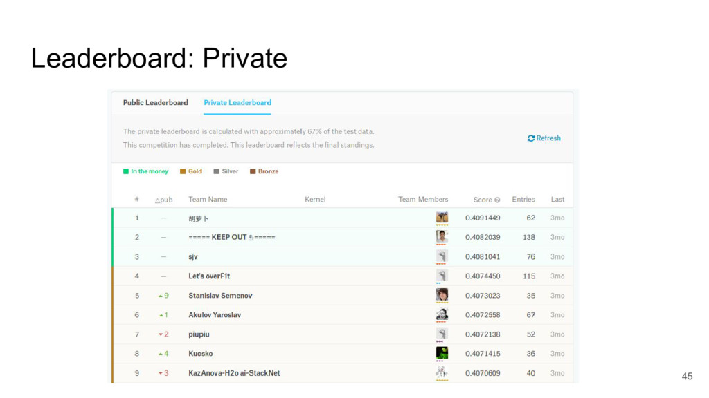
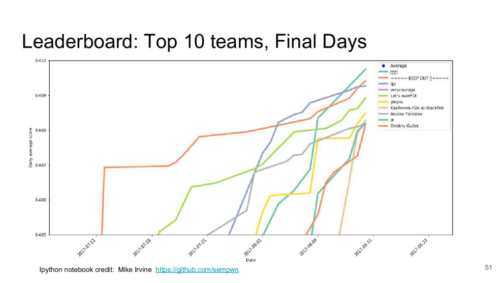
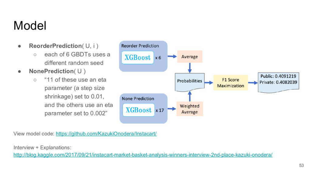
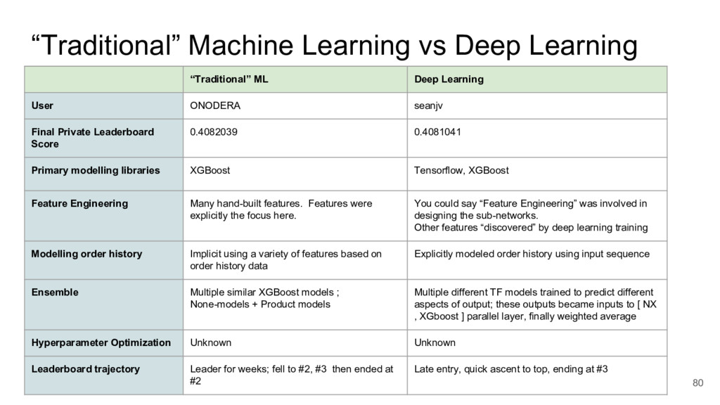
I took a close look at a recent predictive modelling competition on Kaggle.com. The challenge was to predict gocery re-orders on Instacart.com, based on historical data and the particular user’s history.

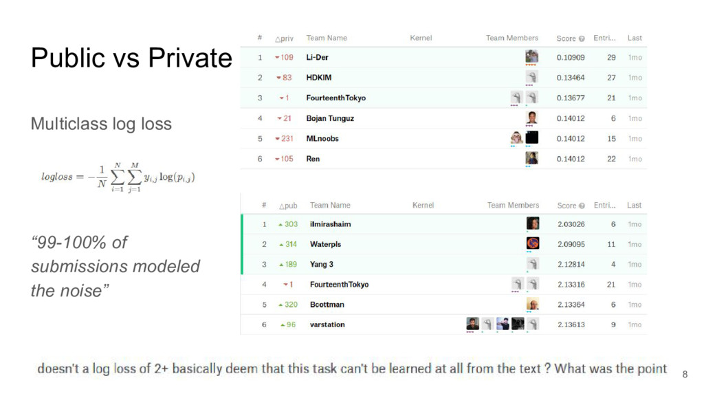
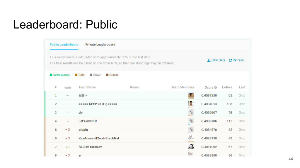
I focused on two submissions, ranked #2 and #3 on the leader board. These two solutions yielded nearly identical scores, using completely different approaches.

These two approaches are emblematic of two approaches to machine learning today.

Transcript

1. Market Basket Analysis
   A Tale of Two Models
   “Traditional” ML vs Deep Learning
   Analysis of https://www.kaggle.com/c/instacart-market-basket-analysis
   By Robin Chauhan robin@pathwayi.com
   

   View Slide

2. ● Robin Ranjit Singh Chauhan https://ca.linkedin.com/in/robinc
   ● Head of Engineering, and Part-time Data Scientist at AgFunder
   ● Founder, Pathway Intelligence Inc
   ● New to kaggle.com and this group (my 3rd sesh)
   ● Indo-Canadian
   ● Live on Sunshine Coast
   ● New here, so grateful to meet people (ie. you).
   ● Would love to hear about what you’re into, both on data science and domain
   sides!
   Who I am
   2
   

   View Slide

3. Credits
   ● Kaggle.com competitors ONODERA and seanvj for sharing their fascinating
   models
   ● Kernel authors on Kaggle.com for sharing their insight
   ● Bruce Sharpe, Mike Irvine, and for their advice in preparing this presentation
   ● Matt Kierans, Charles Iliya Krempeaux, and Bruce Sharpe for organizing
   great data science events in Vancouver
   ● SFU VentureLabs for the meeting space
   3
   

   View Slide

4. - If you understand the Thing
   - better, or in a different way
   - If a Thing is confusing
   - Share an anecdote about using a relate Thing in your domain of
   interest
   - Goal: Mutual Enlightenment
   - Sorry in advance if I get something wrong, please correct me :)
   - I am here to learn
   - After, I would love to hear what I could have improved on
   Requests: Please Share
   4
   

   View Slide

5. Almost picked: Msk Personalized Cancer Treatment
   https://www.kaggle.com/c/msk-redefining-cancer-treatment
   #$%^(#&$ !
   5
   

   View Slide

6. Almost picked: Msk Personalized Cancer Treatment
   goose Y U so angry? #$%^(#&$ !
   6
   

   View Slide

7. Almost picked: Msk Personalized Cancer Treatment
   ● Data leakage
   ● New dataset released 5 days before deadline
   ● Private leaderboard scores were astoundingly worse than public
   ● Suspicion that data was mislabelled
   7
   

   View Slide

8. Public vs Private
   Multiclass log loss
   “99-100% of
   submissions modeled
   the noise”
   8
   

   View Slide

9. View Slide

10. Instacart
    ● US Grocery delivery company
    ● Orders primarily made via phone app + website
    ● “the Most Promising Company in America” -- Forbes in 2015
    ● Allows shopping at in-store prices (delivery charge?)
    ● Investors include Whole Foods (now owned by Amazon...), Y Combinator,
    Sequoia, Khosla, Andreessen H, FundersClub, etc
    ● As of March 2017, Instacart services 36 markets, composed of 1,200 cities in
    25 states (US only atm)
    ● Recently valued at $3.4B (raised $400M in March 2017)
    10
    

    View Slide

11. Instacart - Data Science Stack
    ● Strong programming skills in Python and fluency in data manipulation (SQL, Spark, Pandas) and
    machine learning (scikit-learn, XGBoost, Keras/Tensorflow) tools
    ● Expertise in machine learning for search optimization, discovery driven recommendations, or
    advertising optimization
    ● Expertise in natural language and/or image processing for e-commerce catalog quality,
    enrichment and optimization
    ● Expertise in combining machine learning and operations research to solve optimal routing or
    inventory management problems
    ● Expertise with deep learning methods and their practical application at scale
    ● Writing production applications using Python, R, and SQL
    ● Blog post: Instacart currently uses XGBoost, word2vec and Annoy in production on similar data to
    sort items for users to “buy again”
    ○ Annoy github: Approximate Nearest Neighbors Oh Yeah is a C++ library with Python
    bindings to search for points in space that are close to a given query point
    11
    

    View Slide

12. Goal
    “Currently they use transactional data to develop models that predict which
    products a user will buy again, try for the first time, or add to their cart next during
    a session”
    “use this anonymized data on customer orders over time to predict which [if any]
    previously purchased products will be in a user’s next order”
    Winners get: “cash prize and a fast track through the recruiting process”
    12
    

    View Slide

13. Quirks
    ● Different from the general recommendation problem
    ○ cold start issue of making predictions for new users and new items that we’ve never seen
    before
    ○ Eg. a movie site may need to recommend new movies and make recommendations for brand
    new users
    ● Sequential + temporal aspects
    ○ How do we take the time since a user last purchased an item into account?
    ○ Do users have specific purchase patterns
    ○ Do they buy different kinds of items at different times of the day?
    13
    

    View Slide

14. Vital statistics
    ● $12k, 8k, 5k prizes
    ● Deadline Aug 14, 2017
    ● Submission
    ○ predict a space-delimited list of product_ids for that order.
    ○ If you wish to predict an empty order, you should submit an explicit 'None' value
    order_id,products
    17,1 2
    34,None
    137,1 2 3
    etc.
    14
    

    View Slide

15. Range: 0.0 (worst) to 1.0 (best) inclusive
    Requires both good Precision and Recall
    Implies picking a threshold (unlike AUC) ….
    Evaluation: F1 Metric
    15
    

    View Slide

16. Precision + Recall Refresher
    Q: “How well did we do?” has 2 different answers:
    “Did we succeed in picking
    mostly just green ones?”
    “Out of all the green
    ones, how many did we
    pick?”
    16
    Chart credit: https://commons.wikimedia.org/wiki/User:Walber
    

    View Slide

17. View Slide

18. View Slide

19. The Instacart Online Grocery Shopping Dataset 2017
    ● Anonymized
    ● over 3 million grocery orders from more than 200,000 Instacart users
    ● For each user, between 4 and 100 of their orders, with the sequence of
    products purchased in each order.
    ● the week and hour of day the order was placed
    ● a relative measure of time between orders
    19
    

    View Slide

20. Data
    20
    

    View Slide

21. Orders
    3.4m rows, 206k users
    ● order_id: order identifier
    ● user_id: customer identifier
    ● eval_set: which evaluation set this order belongs in (see SET described
    below)
    ● order_number: the order sequence number for this user (1 = first, n = nth)
    ● order_dow: the day of the week the order was placed on
    ● order_hour_of_day: the hour of the day the order was placed on
    ● days_since_prior: days since the last order, capped at 30 (with NAs for
    order_number = 1)
    21
    

    View Slide

22. Orders
    ● order_products__SET (30m+ rows):
    ○ order_id: foreign key
    ○ product_id: foreign key
    ○ add_to_cart_order: order in which each product was added to cart
    ○ reordered: 1 if this product has been ordered by this user in the past, 0 otherwise
    ● where SET is one of the four following evaluation sets (eval_set in orders):
    ○ "prior": orders prior to that users most recent order (~3.2m orders)
    ○ "train": training data supplied to participants (~131k orders)
    ○ "test": test data reserved for machine learning competitions (~75k orders)
    22
    

    View Slide

23. View Slide

24. Order data
    Prior orders
    Training orders
    Test orders
    24
    

    View Slide

25. 25
    Chart credit: https://www.kaggle.com/sudalairajkumar
    

    View Slide

26. 26
    Chart credit: https://www.kaggle.com/serigne
    

    View Slide

27. 27
    Chart credit: https://www.kaggle.com/sudalairajkumar
    

    View Slide

28. Time of day
    28
    Chart credit: https://www.kaggle.com/philippsp
    

    View Slide

29. Day of week
    29
    Chart credit: https://www.kaggle.com/philippsp
    

    View Slide

30. Day of week + Time
    30
    Chart credit: https://www.kaggle.com/sudalairajkumar
    

    View Slide

31. Order sizes
    31
    Chart credit: https://www.kaggle.com/serigne
    

    View Slide

32. Most Popular Items
    32
    Chart credit: https://www.kaggle.com/philippsp
    

    View Slide

33. When do reorders happen?
    33
    Chart credit: https://www.kaggle.com/sudalairajkumar
    

    View Slide

34. Reorder Frequency
    59% of the ordered
    items are reorders
    34
    Chart credit: https://www.kaggle.com/philippsp
    

    View Slide

35. Per Department Reorder ratio
    35
    Chart credit: https://www.kaggle.com/sudalairajkumar
    

    View Slide

36. Add to cart order vs reorder ratio
    36
    Chart credit: https://www.kaggle.com/sudalairajkumar
    

    View Slide

37. Items in order of
    prob. Reorder
    37
    Chart credit: https://www.kaggle.com/philippsp
    

    View Slide

38. What gets put in
    cart first?
    38
    Chart credit: https://www.kaggle.com/philippsp
    

    View Slide

39. Time of last order vs probability of reorder
    “We can see that if people
    order again on the same day,
    they order the same product
    more often. Whereas when
    30 days have passed, they
    tend to try out new things in
    their order.”
    [Ed: contrast with “when do
    reorders happen” slide where
    30 days is a peak...]
    39
    Chart credit: https://www.kaggle.com/philippsp
    

    View Slide

40. # of orders vs Probability of reordering
    “Products with a high
    number of orders are
    naturally more likely to
    be reordered.
    However, there
    seems to be a ceiling
    effect.”
    40
    Chart credit: https://www.kaggle.com/philippsp
    

    View Slide

41. Organic: fewer sales, higher reorder proportion
    41
    Chart credit: https://www.kaggle.com/philippsp
    

    View Slide

42. By number of products in category
    42
    Chart credit: https://www.kaggle.com/frednavruzov
    

    View Slide

43. By frequency of purchase
    Ed: wish
    placement was
    same :|
    43
    Chart credit: https://www.kaggle.com/frednavruzov
    

    View Slide

44. Leaderboard: Public
    44
    

    View Slide

45. Leaderboard: Private
    45
    

    View Slide

46. Leaderboard
    46
    Ipython notebook credit: Mike Irvine https://github.com/sempwn
    

    View Slide

47. Leaderboard: Daily Averages
    47
    Ipython notebook credit: Mike Irvine https://github.com/sempwn
    

    View Slide

48. Leaderboard: Num subs vs Max Score
    48
    Ipython notebook credit: Mike Irvine https://github.com/sempwn
    

    View Slide

49. Leaderboard: Num Submissions vs Counts
    49
    Ipython notebook credit: Mike Irvine https://github.com/sempwn
    

    View Slide

50. Leaderboard: Top 10 teams
    50
    Ipython notebook credit: Mike Irvine https://github.com/sempwn
    

    View Slide

51. Leaderboard: Top 10 teams, Final Days
    51
    Ipython notebook credit: Mike Irvine https://github.com/sempwn
    

    View Slide

52. 2nd Place: ONODERA
    ● currently in charge of auction services at Yahoo! JAPAN
    52
    

    View Slide

53. Model
    ● ReorderPrediction( U, i )
    ○ each of 6 GBDTs uses a
    different random seed
    ● NonePrediction( U )
    ○ “11 of these use an eta
    parameter (a step size
    shrinkage) set to 0.01,
    and the others use an eta
    parameter set to 0.002”
    53
    View model code: https://github.com/KazukiOnodera/Instacart/
    Interview + Explanations:
    http://blog.kaggle.com/2017/09/21/instacart-market-basket-analysis-winners-interview-2nd-place-kazuki-onodera/
    

    View Slide

54. None Model
    “ One way to think about None is as the probability (1 - Item A) * (1 - Item B) * …
    But another method is to try to predict None as a special case.
    By creating a None model and treating None as just another item, I was able
    to boost my F1 score from 0.400 to 0.407.”
    54
    

    View Slide

55. Data Augmentation
    Used past 3 prior purchases, as
    additional training data
    ”Instead of only using the provided
    training set (“tr”), I also looked a
    short window back in time (the
    cells shaded in yellow) to gather
    more data.”
    55
    

    View Slide

56. Feature Engineering
    “I believe my strength is feature engineering” --ONODERA
    ● User Features
    ● Item Features
    ● ( User, Item ) features
    ● Datetime features
    56
    

    View Slide

57. Feature Importance
    57
    

    View Slide

58. Feature Importance
    ● total_buy_n5(User A, Item B) is the total number of times User A bought Item B out of the 5 most
    recent orders
    ● total_buy_ratio_n5 is the proportion of A's 5 most recent orders in which A bought B [ed: how
    different is that than total_buy_n5?]
    ● useritem_order_days_max_n5, the longest that A has recently gone without buying B.
    ● order_ratio_by_chance_n5 proportion of recent orders in which A had the chance to buy B, and
    did indeed do so.
    ○ A "chance" refers to the number of opportunities the user had for buying the item after first
    encountering it.
    ○ For example, if a user A had order numbers 1-5, and bought item B at order number 2, then
    the user had 4 chances to buy the item at order numbers 2, 3, 4, and 5.)
    ● useritem_order_days_median_n5 is the median number of days that A has recently gone without
    buying B.
    58
    

    View Slide

59. Feature Importance: None Prediction
    59
    

    View Slide

60. ● useritem_sum_pos_cart-mean(User A) whether the user tends to buy a lot
    of items at once.
    ● total_buy-max max number times the user has bought any item.
    ● total_buy_ratio_n5-max is the maximum proportion of the 5 most recent
    orders in which the user bought a certain item. Eg, if there was an item the
    user bought in 4 out of their 5 most recent orders, but no other item more
    often than that, this feature would be 0.8.
    ● total_buy-mean mean number of times the user has bought any item.
    ● t-1_reordered_ratio proportion of items in the previous order that were
    repurchases.
    Feature Importance: None Prediction
    60
    

    View Slide

61. Insight: When user does *not* order
    “This user pretty
    much always orders
    Cola. But at order
    number 8, the user
    didn’t. Why not?
    Probably because
    the user bought
    Fridge Pack Cola
    instead.”
    61
    

    View Slide

62. Insight: days_last_order-max
    Days_since_last_order_this_item(U
    ser A, Item B) # of days since User A
    last ordered Item B
    Useritem_orders_days_max(User A,
    Item B) max of the above feature
    across time, i.e., the longest that User
    A has ever gone without ordering B.
    Days_last_order-max(User A, Item
    B) diff between these two. How ready
    the user is to repurchase the item.
    62
    

    View Slide

63. Initial grid search for global
    p_min yielded 0.2.
    Discussion about how order
    should have its own
    threshold, code from Faron
    Row 1: We should predict
    that Item A and only Item A
    will be reordered. Need a
    threshold between 0.3 and
    0.9.
    Row 2: optimal choice is to
    predict that Items A and B
    will both be reordered.
    Needs threshold less than
    0.2 (the probability that Item
    B will be reordered)
    F1 Maximization
    Model predictions are
    Model predictions are
    Our submission is...
    Our expected F1 for this (repeated/average) case...
    Our submission is...
    63
    

    View Slide

64. F1 Maximization: Threshold Selection
    “So each order should have its own threshold.
    To determine this threshold I wrote a simulation
    algorithm as follows.
    Simulate 10k itemsets using probabilities from model…”
    64
    

    View Slide

65. F1 Maximization: Threshold Selection
    Calculate the expected F1 score
    for each set of labels, starting
    from the highest probability items
    Add items (e.g., [A], then [A, B],
    then [A, B, C], etc) until the F1
    score peaks and then decreases
    [ed: at time of prediction]
    65
    

    View Slide

66. 3rd Place: seanjv
    ● Deep learning (plus lightgbm)!
    ● Tensorflow (no keras)
    ● Polar opposite of ONODERA solution: little feature engineering
    ● Github: “Student at MIT”
    ● https://github.com/sjvasquez/instacart-basket-prediction
    66
    

    View Slide

67. Top Level Architecture
    Product: RNN w/LSTM,
    Wavenet CNN
    Aisle RNN
    Dept RNN
    Product RNN Bernoulli mixture
    model
    Order size RNN
    Order size RNN mixture model
    Skipgram w/neg sampling
    NNMF
    lightgbm
    FF NN
    (2 layer, 1 skip)
    Wtd avg ;
    F1 max
    Inputs
    67
    Diagram credit: Robin Chauhan robin@pathwayi.com
    

    View Slide

68. Deep learning solution: First level
    ● Product RNN/CNN (code): a combined RNN and CNN trained to predict the probability that a user
    will order a product at each timestep. The RNN is a single-layer LSTM and the CNN is a 6-layer
    causal CNN with dilated convolutions.
    ● Aisle RNN (code): an RNN similar to the first model, but trained at the aisle level (predict whether a
    user purchases any products from a given aisle at each timestep).
    ● Department RNN (code): an RNN trained at the department level.
    ● Product RNN mixture model (code): an RNN similar to the first model, but instead trained to
    maximize the likelihood of a bernoulli mixture model.
    ● Order size RNN (code): an RNN trained to predict the next order size, minimizing RMSE.
    ● Order size RNN mixture model (code): an RNN trained to predict the next order size, maximizing
    the likelihood of a gaussian mixture model.
    ● Skip-Gram with Negative Sampling (SGNS) (code): SGNS trained on sequences of ordered
    products.
    ● Non-Negative Matrix Factorization (NNMF) (code): NNMF trained on a matrix of user-product
    order counts. 68
    

    View Slide

69. Product RNN/CNN: Detail
    Wavenet:
    6 layer dilated
    causal
    convolutions
    LSTM layer
    TDDL
    relu
    Inputs TDDL
    sigmoid
    69
    Diagram credit: Robin Chauhan robin@pathwayi.com
    

    View Slide

70. Product RNN/CNN
    h = lstm_layer(x, self.history_length, self.lstm_size)
    # wavenet: time_distributed_dense_layer, multiple (6) temporal_convolution_layers ,
    # then time_distributed_dense_layer
    c = wavenet(x, self.dilations, self.filter_widths, self.skip_channels, self.residual_channels)
    h = tf.concat([h, c, x], axis=2) # wavenet(x) and lstm(x) in parallel with x
    # time_distributed_dense_layer: Applies a shared dense layer to each timestep of a tensor of shape
    # [batch_size, max_seq_len, input_units]
    self.h_final = time_distributed_dense_layer(h, 50, activation=tf.nn.relu, scope='dense-1')
    y_hat = time_distributed_dense_layer(self.h_final, 1, activation=tf.nn.sigmoid,
    scope='dense-2')
    y_hat = tf.squeeze(y_hat, 2)
    70
    

    View Slide

71. Product RNN/CNN: Inputs
    def get_input_sequences(self):
    self.user_id = tf.placeholder(tf.int32, [None])
    self.product_id = tf.placeholder(tf.int32, [None])
    self.aisle_id = tf.placeholder(tf.int32, [None])
    self.department_id = tf.placeholder(tf.int32, [None])
    self.is_none = tf.placeholder(tf.int32, [None])
    self.history_length = tf.placeholder(tf.int32, [None])
    self.is_ordered_history = tf.placeholder(tf.int32, [None, 100]) # Note dimensions
    self.index_in_order_history = tf.placeholder(tf.int32, [None, 100])
    self.order_dow_history = tf.placeholder(tf.int32, [None, 100])
    self.order_hour_history = tf.placeholder(tf.int32, [None, 100])
    self.days_since_prior_order_history = tf.placeholder(tf.int32, [None, 100])
    self.order_size_history = tf.placeholder(tf.int32, [None, 100])
    self.reorder_size_history = tf.placeholder(tf.int32, [None, 100])
    self.order_number_history = tf.placeholder(tf.int32, [None, 100])
    self.product_name = tf.placeholder(tf.int32, [None, 30])
    self.product_name_length = tf.placeholder(tf.int32, [None])
    self.next_is_ordered = tf.placeholder(tf.int32, [None, 100])
    ….. 71
    

    View Slide

72. Product RNN/CNN: Wavenet
    def wavenet(x, dilations, filter_widths, skip_channels, residual_channels, scope='wavenet', reuse=False):
    """
    A stack of causal dilated convolutions with paramaterized residual and skip connections as
    described in the WaveNet paper (with some minor differences).
    ….
    72
    

    View Slide

73. Aside: Wavenet
    73
    Diagram credit: https://www.slideshare.net/xavigiro/speech-synthesis-wavenet-d4l1-deep-learning-for-speech-and-language-upc-2017
    

    View Slide

74. TDDL: time_distributed_dense_layer
    def time_distributed_dense_layer(inputs, output_units, bias=True, activation=None, batch_norm=None,
    dropout=None, scope='time-distributed-dense-layer', reuse=False):
    """
    Applies a shared dense layer to each timestep of a tensor of shape [batch_size, max_seq_len, input_units]
    to produce a tensor of shape [batch_size, max_seq_len, output_units].
    Args:
    inputs: Tensor of shape [batch size, max sequence length, ...].
    output_units: Number of output units.
    activation: activation function.
    dropout: dropout keep prob.
    Returns:
    Tensor of shape [batch size, max sequence length, output_units].
    """
    74
    

    View Slide

75. Product RNN/CNN: Embeddings
    product_embeddings = tf.get_variable(
    name='product_embeddings',
    shape=[50000, self.lstm_size],
    dtype=tf.float32
    )
    aisle_embeddings = tf.get_variable(
    name='aisle_embeddings',
    shape=[250, 50],
    dtype=tf.float32
    )
    department_embeddings = tf.get_variable(
    name='department_embeddings',
    shape=[50, 10],
    dtype=tf.float32
    )
    user_embeddings = tf.get_variable(
    name='user_embeddings',
    shape=[207000, self.lstm_size],
    dtype=tf.float32
    )
    75
    

    View Slide

76. Deep learning solution: Second level
    ● GBM (code): a lightgbm model.
    ● Feedforward NN (code): a feedforward neural network.
    The final reorder probabilities are a weighted average of the outputs from the second-level models.
    The final basket is chosen by using these probabilities and choosing the product subset with maximum
    expected F1-score.
    76
    

    View Slide

77. Other solutions
    ● CatBoost popular
    ● Some users isolated the most popular products
    ● Association rule learning (mlextend), moving averages, moments of
    distributions
    ● “you can do (almost) anything in pandas in reasonable time if you spend
    enough time on planning and vectorizing” -- Kucsko
    ○ “we could do a groupby user+product apply diff, however this is extremely slow.
    ○ instead we can be a bit clever and do a groupby user+product shift and then take the
    difference between the shifted an unshifted vector.
    ○ after that we can easily take mean, med, std etc
    77
    

    View Slide

78. Words of wisdom from ONODERA
    What have you taken away from this competition?
    All metrics can be hacked, I think. Especially metrics where
    we have to convert probabilities to binary scores. (Although
    metrics like AUC are rarely hacked.)
    78
    

    View Slide

79. Words of wisdom from ONODERA
    Do you have any advice for those just getting started in data
    science?
    Join the competitions you like. But never give up before the end, and try
    every approach you come up with. I know it’s a tradeoff between sleep
    and your leaderboard ranking. It’s common for features that take a lot of
    time to construct to wind up doing nothing. But we can’t know the result if
    we don't do anything. So the most important thing is to participate in
    the delusion that you’ll get a better result if you try!
    79
    

    View Slide

80. “Traditional” Machine Learning vs Deep Learning
    80
    “Traditional” ML Deep Learning
    User ONODERA seanjv
    Final Private Leaderboard
    Score
    0.4082039 0.4081041
    Primary modelling libraries XGBoost Tensorflow, XGBoost
    Feature Engineering Many hand-built features. Features were
    explicitly the focus here.
    You could say “Feature Engineering” was involved in
    designing the sub-networks.
    Other features “discovered” by deep learning training
    Modelling order history Implicit using a variety of features based on
    order history data
    Explicitly modeled order history using input sequence
    Ensemble Multiple similar XGBoost models ;
    None-models + Product models
    Multiple different TF models trained to predict different
    aspects of output; these outputs became inputs to [ NX
    , XGboost ] parallel layer, finally weighted average
    Hyperparameter Optimization Unknown Unknown
    Leaderboard trajectory Leader for weeks; fell to #2, #3 then ended at
    #2
    Late entry, quick ascent to top, ending at #3
    

    View Slide