Chien-Liu Lin

Transcript

1. MRC | Medical Research Council Improving the precision of oncology trials analysis using progression-free-survival as an endpoint Chien-Ju Lin and James Wason Medical Research Council
2. MRC | Medical Research Council Fixed time Best observed response (BOR) Time to event
3. MRC | Medical Research Council What is tumour size measurement Baseline (z0 ): 10cm Follow-up(zt ): 6cm Taken from Nishino et at. DOI: 10.2214/AJR.09.4110
4. MRC | Medical Research Council What is RECIST (Response Evaluation Criteria in Solid Tumours) 0 Complete Response 0.7 ( ↓30%) 1.2 (↑ 20%) Partial Response Progressive Disease Stable Disease Ratio zt /z0 • tumour progression • new-lesion progression
5. MRC | Medical Research Council t0 : Baseline follow-up proportion of responder at the fixed time { } { } patients # lesions new no & 0.7 shrinkage tumour with patients # > =
6. MRC | Medical Research Council Binary method ü simplify data analysis and interpretation of results o loss of information 0.7 ( ↓30%) 1.2 (↑ 20%) 35% v.s. 25%
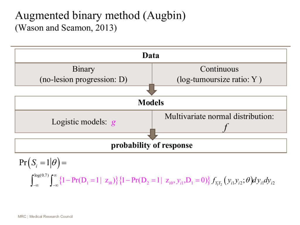
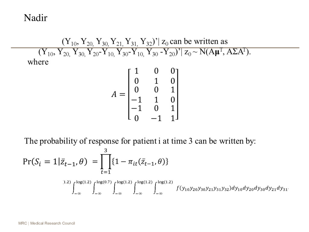
7. MRC | Medical Research Council Augmented binary method (Augbin) (Wason and Seamon, 2013) Data Binary (no-lesion progression: D) Continuous (log-tumoursize ratio: Y ) Models Logistic models: g Multivariate normal distribution: probability of response f ( ) Pr 1 i S q = = { }{ } ( ) 1 2 log(0.7 1 i0 2 i0 1 1 ) 1 2 1 2 1 Pr(D 1| z ) 1 Pr(D 1| z , ,D 0 ; ) YY i i i i i f y y dy dy y q ¥ -¥ -¥ - = - = = ò ò
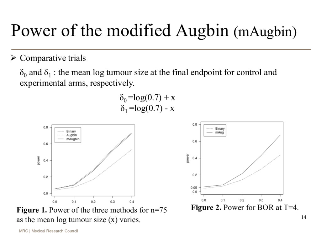
8. MRC | Medical Research Council Power of the modified Augbin (mAugbin) Ø Comparative trials δ0 and δ1 : the mean log tumour size at the final endpoint for control and experimental arms, respectively. δ0 =log(0.7) + x δ1 =log(0.7) - x Figure 1. Power of the three methods for n=75 as the mean log tumour size (x) varies. Figure 2. Power for BOR at T=4. 14
9. MRC | Medical Research Council
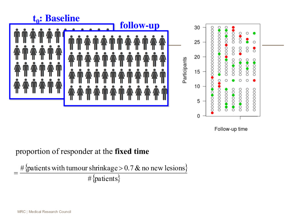
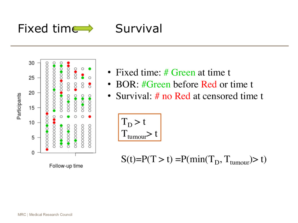
10. MRC | Medical Research Council Fixed time Survival • Fixed time: # Green at time t • BOR: #Green before Red or time t • Survival: # no Red at censored time t S(t)=P(T > t) =P(min(TD , Ttumour )> t) TD > t Ttumour > t
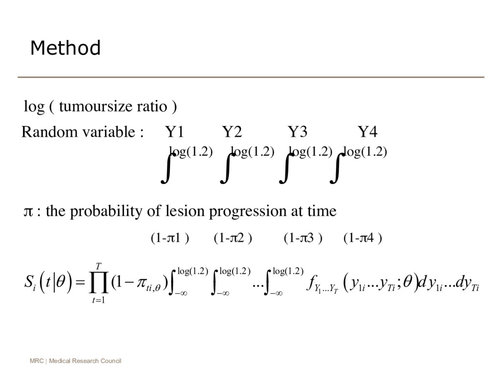
11. MRC | Medical Research Council ( ) ( ) 1 log(1.2) log(1.2) log(1.2) , ... 1 1 1 (1 ) ... ... ; ... T T i ti Y Y i Ti i Ti t S t f y y dy dy q q p q -¥ -¥ -¥ = = - Õ ò ò ò ∫ ∫ ∫ ∫ Random variable : Y1 Y2 Y3 Y4 (1-π1 ) (1-π2 ) (1-π3 ) (1-π4 ) π : the probability of lesion progression at time log ( tumoursize ratio ) Method log(1.2) log(1.2) log(1.2) log(1.2)
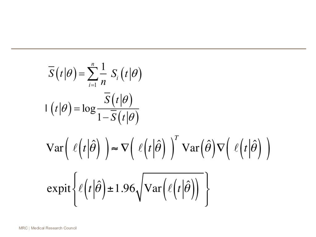
12. MRC | Medical Research Council ( ) i S t q ( ) 1 1 n i S t n q = = å ( ) ( ) ( ) log 1 S t t S t q q q = - l Var ℓ t ˆ θ ( ) ( )≈ ∇ ℓ t ˆ θ ( ) ( )T Var ˆ θ ( )∇ ℓ t ˆ θ ( ) ( ) expit ℓ t ˆ θ ( )±1.96 Var ℓ t ˆ θ ( ) ( ) ⎧ ⎨ ⎪ ⎩ ⎪ ⎫ ⎬ ⎪ ⎭ ⎪
13. MRC | Medical Research Council
14. MRC | Medical Research Council
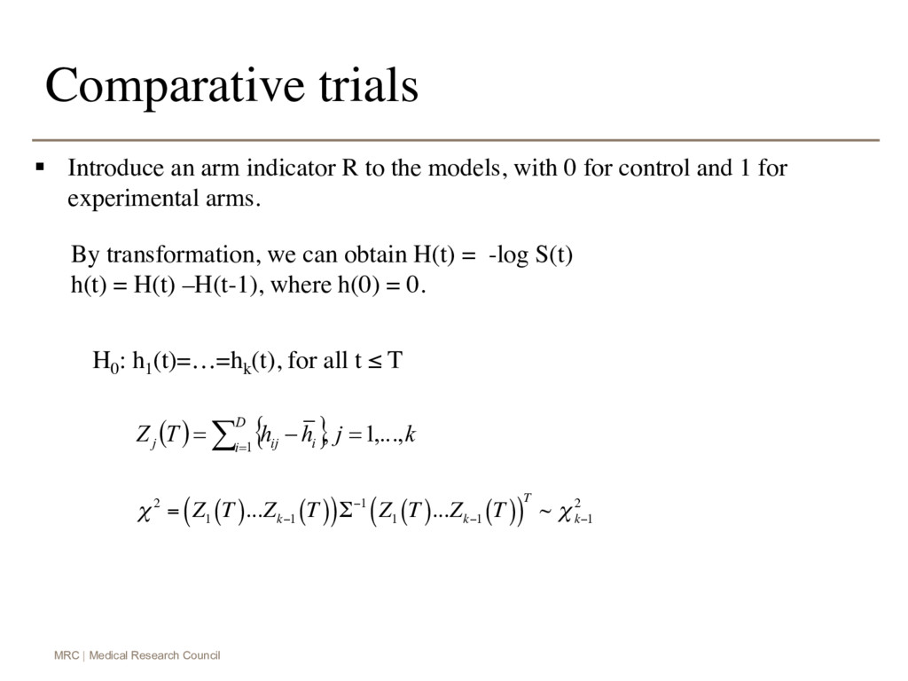
15. MRC | Medical Research Council Comparative trials By transformation, we can obtain H(t) = -log S(t) h(t) = H(t) –H(t-1), where h(0) = 0. § Introduce an arm indicator R to the models, with 0 for control and 1 for experimental arms. H0 : h1 (t)=…=hk (t), for all t ≤ T ( ) { } k j h h T Z D i i ij j ,..., 1 , 1 = - = å = χ2 = Z 1 T ( )...Z k−1 T ( ) ( )Σ−1 Z 1 T ( )...Z k−1 T ( ) ( )T ~ χ2 k−1
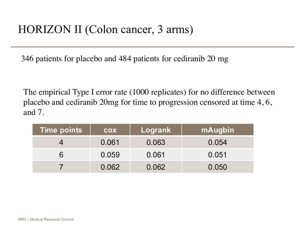
16. MRC | Medical Research Council HORIZON II (Colon cancer, 3 arms) Time points cox Logrank mAugbin 4 0.061 0.063 0.054 6 0.059 0.061 0.051 7 0.062 0.062 0.050 346 patients for placebo and 484 patients for cediranib 20 mg The empirical Type I error rate (1000 replicates) for no difference between placebo and cediranib 20mg for time to progression censored at time 4, 6, and 7.
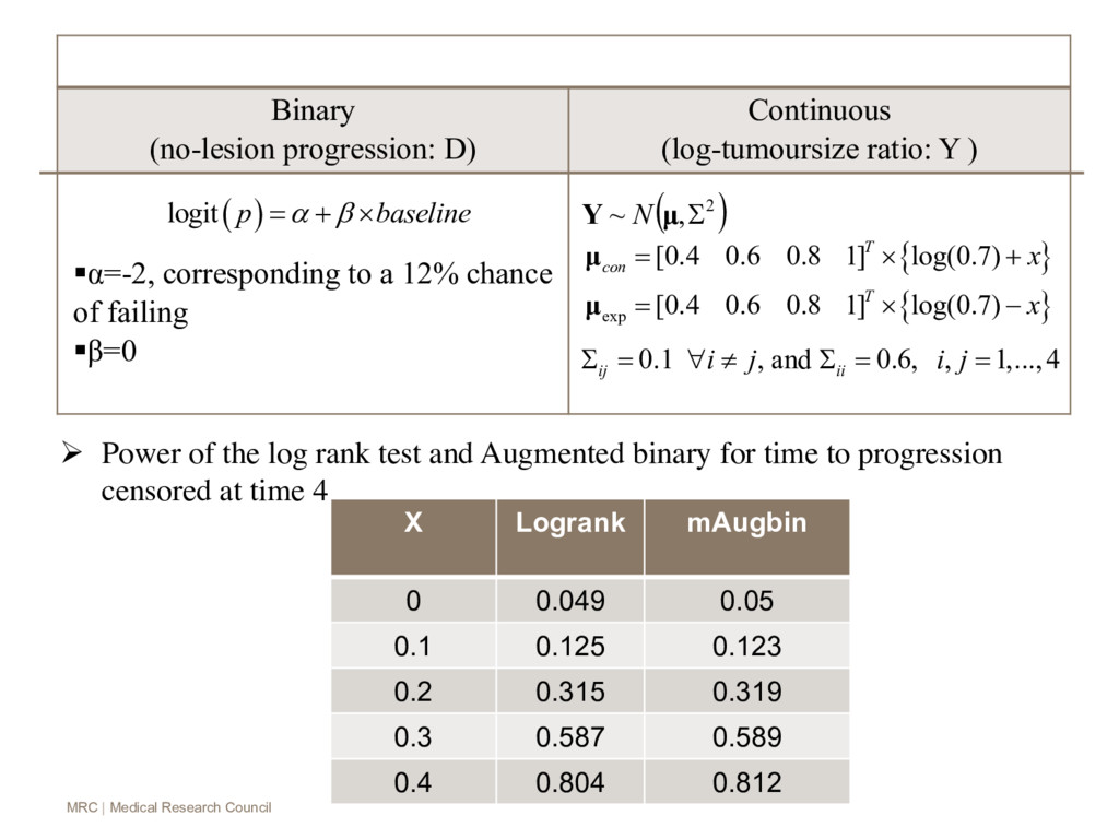
17. MRC | Medical Research Council Ø Power of the log rank test and Augmented binary for time to progression censored at time 4 { } { } exp [0.4 0.6 0.8 1] log(0.7) [0.4 0.6 0.8 1] log(0.7) T con T x x = ´ + = ´ - µ µ 0.1 , and 0.6, , 1,...,4 ij ii i j i j S = " ¹ S = = Binary (no-lesion progression: D) Continuous (log-tumoursize ratio: Y ) §α=-2, corresponding to a 12% chance of failing §β=0 ( ) logit p baseline a b = + ´ X Logrank mAugbin 0 0.049 0.05 0.1 0.125 0.123 0.2 0.315 0.319 0.3 0.587 0.589 0.4 0.804 0.812 ( ) 2 , ~ S µ Y N
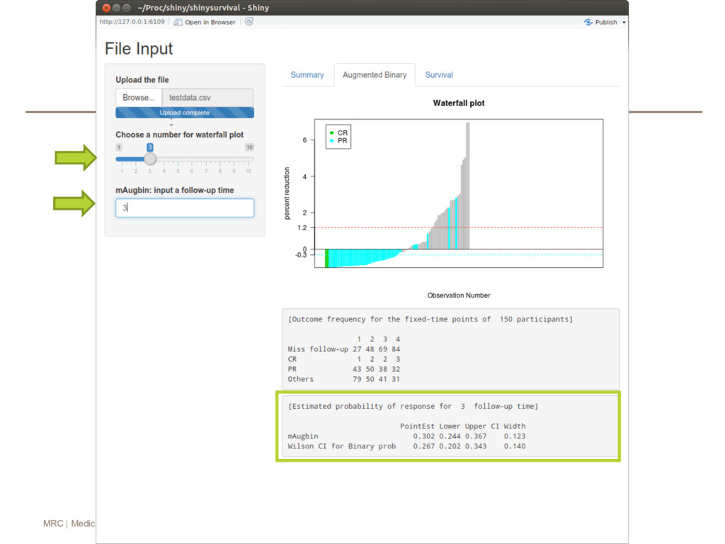
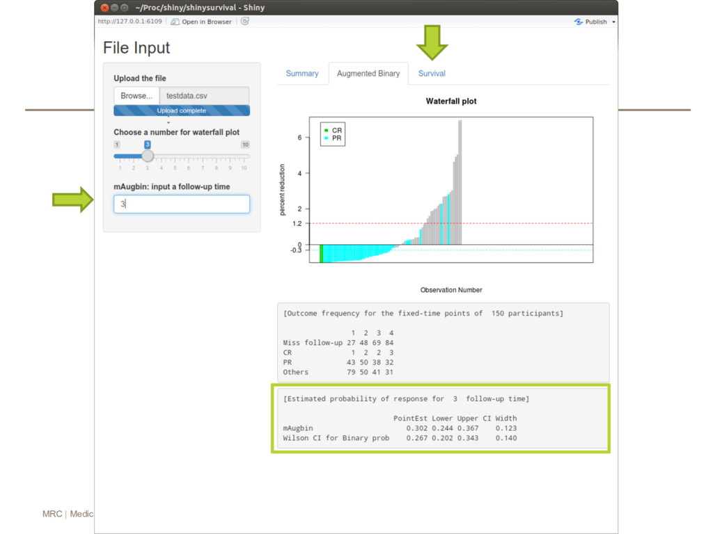
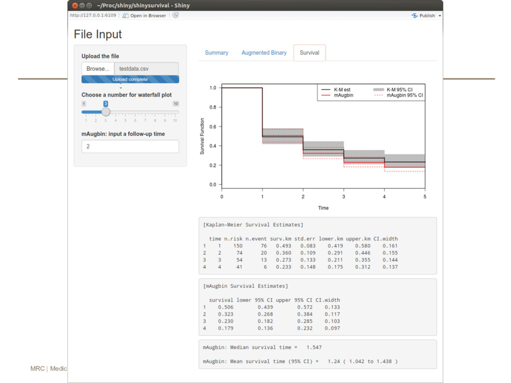
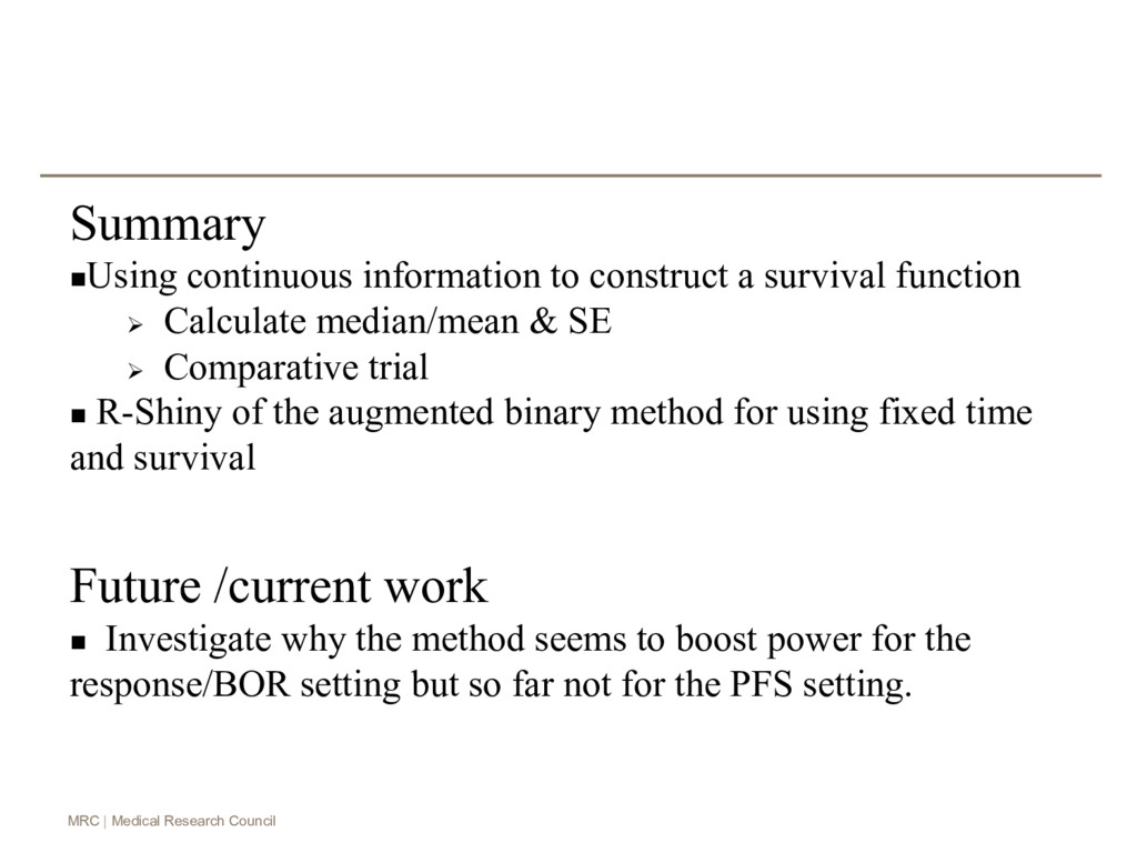
18. MRC | Medical Research Council Summary nUsing continuous information to construct a survival function Ø Calculate median/mean & SE Ø Comparative trial n R-Shiny of the augmented binary method for using fixed time and survival Future /current work n Investigate why the method seems to boost power for the response/BOR setting but so far not for the PFS setting.
19. MRC | Medical Research Council Thank You
20. MRC | Medical Research Council Nadir