Prospects For Near-future Detection & Astrophysical Inference With Pulsar-timing Arrays

Stephen Taylor CaJAGWR seminar, 12-01-2015 © 2015 California Institute of
Technology. Government sponsorship acknowledged PROSPECTS FOR NEAR-FUTURE Stephen R. Taylor GRAVITATIONAL-WAVE DETECTION & ASTROPHYSICAL INFERENCE WITH PULSAR-TIMING ARRAYS NASA POSTDOCTORAL FELLOW, JET PROPULSION LABORATORY

Stephen Taylor CaJAGWR seminar, 12-01-2015 Pulsars and pulsar timing Searching
for gravitational waves by timing pulsars Pursuing gravitational-wave detection by timing pulsars Sources, spectrum, and state-of-the-art constraints Near-future prospects for detection, and inﬂuence of binary environments Overview

Stephen Taylor CaJAGWR seminar, 12-01-2015 1012 Discovered in 1967 by
Hewish, Bell, et al. Rapid rotation (P~1s), and strong magnetic field (~ G) Radio emission along magnetic field axis Misalignment of rotation and magnetic field axes creates lighthouse effect Pulsars Image credit: Bill Saxton

Stephen Taylor CaJAGWR seminar, 12-01-2015 Millisecond Pulsars Discovered in 1982
with a rotational period of ~1.6 ms Diminished magnetic ﬁeld but much faster rotational frequency They have accreted material from a companion star (they are “recycled”) R o t a t i o n a l s t a b i l i t y w a s comparable to atomic clocks

Stephen Taylor CaJAGWR seminar, 12-01-2015 pulsar timing tests of GR
probes of ISM investigations of nuclear matter ﬁrst exoplanet detection

Stephen Taylor CaJAGWR seminar, 12-01-2015 pulsar timing tests of GR
probes of ISM investigations of nuclear matter ﬁrst exoplanet detection gravitational waves

Stephen Taylor CaJAGWR seminar, 12-01-2015

Stephen Taylor CaJAGWR seminar, 12-01-2015 Searching for GWs with pulsar
timing Detector is an Earth-pulsar system with ~kpc separation Gravitational wave deforms space-time between Earth and pulsar Alters proper separation of Earth and pulsar Pulses are either advanced or delayed with respect to predictions based on deterministic timing-model

Stephen Taylor CaJAGWR seminar, 12-01-2015 John Rowe Animation/Australia Telescope National
Facility, CSIRO

Stephen Taylor CaJAGWR seminar, 12-01-2015 Primary candidate signal is a
stochastic background of GWs Induces stochastic variations in pulse arrival time (TOA) with signiﬁcant low-frequency structure We can’t just look for the spectral signature of GW background, since other intrinsic pulsar processes may look similar (e.g. some pulsars exhibit strong red noise features) Searching for GWs with pulsar timing

Stephen Taylor CaJAGWR seminar, 12-01-2015 Primary candidate signal is a
stochastic background of GWs Induces stochastic variations in pulse arrival time (TOA) with signiﬁcant low-frequency structure We can’t just look for the spectral signature of GW background, since other intrinsic pulsar processes may look similar (e.g. some pulsars exhibit strong red noise features) Searching for GWs with pulsar timing WE DON’T TIME JUST ONE PULSAR, WE TIME MANY PULSAR TIMING ARRAY

Stephen Taylor CaJAGWR seminar, 12-01-2015 Detecting GWs with pulsar timing
hsa(t)⇤sb(t0)i = abC(|t t0|)

Overlap reduction function hsa(t)⇤sb(t0)i = abC(|t t0|)

Overlap reduction function We form a detection statistic based on the expected spatial correlation signature Gaussian-stationary, unpolarized isotropic stochastic GW background has distinctive signature — “Hellings and Downs” curve hsa(t)⇤sb(t0)i = abC(|t t0|)

We form a detection statistic based on the expected spatial correlation signature Gaussian-stationary, unpolarized isotropic stochastic GW background has distinctive signature — “Hellings and Downs” curve Smoking-gun for detection Pa r a m e t r i ze d ove r l a p reduction function can be used to probe anisotropy of the nHz GW sky [Mingarelli (2013), Taylor & Gair (2013), Taylor, Mingarelli, et al. (2015)] Hellings & Downs (1983)

Stephen Taylor CaJAGWR seminar, 12-01-2015 Sources & Spectrum Sensitivity band
set by total observation time (1/decades) and observational cadence (1/weeks) — [ ~ 1- 100 nHz ] Primary candidate is population of supermassive black-hole binaries

set by total observation time (1/decades) and observational cadence (1/weeks) — [ ~ 1- 100 nHz ] Primary candidate is population of supermassive black-hole binaries Image credit: CSIRO

set by total observation time (1/decades) and observational cadence (1/weeks) — [ ~ 1- 100 nHz ] Primary candidate is population of supermassive black-hole binaries Other sources in the nHz band may be decaying cosmic-string networks, or relic GWs from the early Universe Image credit: CSIRO

Stephen Taylor CaJAGWR seminar, 12-01-2015 Sources & Spectrum Supermassive black
hole binaries (SMBHBs) are thought to form ubiquitously within models of galaxy formation Supermassive black holes are copious in the nuclei of nearby galaxies Several relationships exhibit coevolution between galactic bulge properties and the central black hole Current paradigm of galaxy formation is that galaxies undergo repeated merger events, and accrete from cosmic web ﬁlaments (White & Rees, 1978) DeLucia & Blaizot (2007)

Stephen Taylor CaJAGWR seminar, 12-01-2015 “Final parsec problem” Dynamical friction
not a sufﬁcient driving mechanism to induce merger within a Hubble time e.g., Milosavljevic & Merritt (2003) Sources & Spectrum

Stephen Taylor CaJAGWR seminar, 12-01-2015 “Final parsec problem” Dynamical friction
not a sufﬁcient driving mechanism to induce merger within a Hubble time e.g., Milosavljevic & Merritt (2003) Additional environmental couplings may extract energy and angular momentum from binary to drive it to sub-pc separations Sources & Spectrum

Stephen Taylor CaJAGWR seminar, 12-01-2015 Sources & Spectrum stellar scattering
Slingshots of stars from within dense galactic core can extract energy/ angular-momentum from orbit [ e.g. Quinlan (1996) ] “Loss cone” describes phase space of centrophilic stellar orbits A binary may deplete loss cone before it reaches sub-pc separations Asymmetry or triaxiality of stellar bulge can ensure loss cone is topped up

Stephen Taylor CaJAGWR seminar, 12-01-2015 Sources & Spectrum Circumbinary accretion
disks can form around the binary This disk exerts a torque on the b i n a r y, e x t r a c t i n g a n g u l a r momentum and energy, driving the black holes together [ e.g. Ivanov, Papaloizou, Polnarev (1999) ] circumbinary disk interaction

Stephen Taylor CaJAGWR seminar, 12-01-2015 binary eccentricity Sources & Spectrum
An increase in binary eccentricity can be a by-product of the two former mechanisms Eccentric systems emit a spectrum of harmonics of the orbital frequency System is driven to smaller orbital separations faster than a corresponding circular system B 1232 P. C. P E w p f lO g S a IO T T .2 .6 e, — = ,8 Peters (1964)

Stephen Taylor CaJAGWR seminar, 12-01-2015 Sources & Spectrum How do
we build a stochastic signal from these binaries, and how do the different physical processes affect the spectrum?

we build a stochastic signal from these binaries, and how do the different physical processes affect the spectrum? h2 c (f) = Z 1 0 dz Z 1 0 dM1 Z 1 0 dq d4N dzdM1dqdtr dtr d ln fK,r ⇥h2(fK,r) 1 X n=1 g[n, e(fK,r)] (n/2)2  f nfK,r (1 + z) Phinney (2001), Sesana (2013)

we build a stochastic signal from these binaries, and how do the different physical processes affect the spectrum? h2 c (f) = Z 1 0 dz Z 1 0 dM1 Z 1 0 dq d4N dzdM1dqdtr dtr d ln fK,r ⇥h2(fK,r) 1 X n=1 g[n, e(fK,r)] (n/2)2  f nfK,r (1 + z) Phinney (2001), Sesana (2013) (a) (b) (c) (a) Comoving merger rate — affects overall signal level (b)Binary evolution — affects shape of spectrum through time binaries spend emitting at each frequency (binary environmental inﬂuences enter here) (c) Eccentricity — affects shape of spectrum through binary orbital evolution

we build a stochastic signal from these binaries, and how do the different physical processes affect the spectrum? h2 c (f) = Z 1 0 dz Z 1 0 dM1 Z 1 0 dq d4N dzdM1dqdtr dtr d ln fK,r ⇥h2(fK,r) 1 X n=1 g[n, e(fK,r)] (n/2)2  f nfK,r (1 + z) Phinney (2001), Sesana (2013) Circular, GW-driven population — Binaries coupled to stellar population — hc(f) / f 2/3 hc(f) / f hc(f) / f 2/3 low-f high- f

Stephen Taylor CaJAGWR seminar, 12-01-2015 circumbinary disk interaction stellar hardening
binary eccentricity 10-9 10-8 10-7 f [Hz] 10-15 10-14 hc(f) hc( f = 1yr-1) = A = 1⇥10-15 T = 9 yrs

binary eccentricity 10-9 10-8 10-7 f [Hz] 10-15 10-14 hc(f) hc( f = 1yr-1) = A = 1⇥10-15 T = 9 yrs 10-9 10-8 10-7 f [Hz] 10-15 10-14 hc(f) hc( f = 1yr-1) = A = 1⇥10-15 T = 11 yrs

binary eccentricity 10-9 10-8 10-7 f [Hz] 10-15 10-14 hc(f) hc( f = 1yr-1) = A = 1⇥10-15 T = 9 yrs 10-9 10-8 10-7 f [Hz] 10-15 10-14 hc(f) hc( f = 1yr-1) = A = 1⇥10-15 T = 11 yrs 10-9 10-8 10-7 f [Hz] 10-15 10-14 hc(f) hc( f = 1yr-1) = A = 1⇥10-15 T = 15 yrs

binary eccentricity 10-9 10-8 10-7 f [Hz] 10-15 10-14 hc(f) hc( f = 1yr-1) = A = 1⇥10-15 T = 9 yrs 10-9 10-8 10-7 f [Hz] 10-15 10-14 hc(f) hc( f = 1yr-1) = A = 1⇥10-15 T = 11 yrs 10-9 10-8 10-7 f [Hz] 10-15 10-14 hc(f) hc( f = 1yr-1) = A = 1⇥10-15 T = 15 yrs 10-9 10-8 10-7 f [Hz] 10-15 10-14 hc(f) hc( f = 1yr-1) = A = 1⇥10-15 T = 30 yrs

Stephen Taylor CaJAGWR seminar, 12-01-2015 State of the art PROBE
ANISOTROPY THROUGH ORF

Stephen Taylor CaJAGWR seminar, 12-01-2015 State of the art population
courtesy of A. Sesana PROBE ANISOTROPY THROUGH ORF

Stephen Taylor CaJAGWR seminar, 12-01-2015 1.6 2.4 3.2 4.0 4.8
5.6 6.4 A95% ul h ( ˆ ⌦) [⇥10 14] Taylor et al. (2015), PRL State of the art PROBE ANISOTROPY THROUGH ORF

Stephen Taylor CaJAGWR seminar, 12-01-2015 Upper limits reference the characteristic
strain amplitude at a GW frequency of 1/yr (~32 nHz) . 3.0 ⇥ 10 15 State of the art Environmental Coupling • Stellar hardening • Gas-driven inspiral • Eccentricity Galaxy Population Uncertainties • Merger timescale • SMBH - host relations • Pair fraction • Redshift evolution Diminished GW Signal • BSMBH stalling • GW absorption Characteristic strain, hc 1E-17 1E-16 1E-15 1E-14 1E-13 1E-12 Gravitational Wave Frequency, f (Hz) 1E-10 1E-09 1E-08 1E-07 1E-06 hc f 10.— A conceptual view of how various uncertainties in the BSMBH population and the GWs we can Burke-Spolaor (2015)

Stephen Taylor CaJAGWR seminar, 12-01-2015 Upper limits reference the characteristic
strain amplitude at a GW frequency of 1/yr (~32 nHz) . 3.0 ⇥ 10 15 State of the art Environmental Coupling • Stellar hardening • Gas-driven inspiral • Eccentricity Galaxy Population Uncertainties • Merger timescale • SMBH - host relations • Pair fraction • Redshift evolution Diminished GW Signal • BSMBH stalling • GW absorption Characteristic strain, hc 1E-17 1E-16 1E-15 1E-14 1E-13 1E-12 Gravitational Wave Frequency, f (Hz) 1E-10 1E-09 1E-08 1E-07 1E-06 hc f 10.— A conceptual view of how various uncertainties in the BSMBH population and the GWs we can Final- parsec physics Merger rate, BH-galaxy relationshi ps Burke-Spolaor (2015)

Stephen Taylor CaJAGWR seminar, 12-01-2015 Lentati, Taylor, Mingarelli et al.
(2015) Shannon et al. (2015) Arzoumanian et al. (2015) [led by Ellis, inc. Taylor, Mingarelli, van Haasteren, Vallisneri, Lazio] Upper limits reference the characteristic strain amplitude at a GW frequency of 1/yr (~32 nHz) . 1.5 ⇥ 10 15 . 3.0 ⇥ 10 15 . 1.0 ⇥ 10 15 State of the art Characteristic amplitude, A1yr Year First MSP discovered 1e-16 1e-15 1e-14 1e-13 1e-12 1980 1985 1990 1995 2000 2005 2010 2015 2020 Predicted BSMBH Background Fig. 5.— Upper limits on the power-law GWB for a spectral index ↵ = 2/3. Limits improved steadily after dedicated timing of millisecond pul- Burke-Spolaor (2015)

Stephen Taylor CaJAGWR seminar, 12-01-2015 Simultaneously ﬁt for stochastic GW
background, correlated clock-noise, dipole process due to imprecise solar-system ephemerides, and intrinsic low- frequency pulsar noise. Investigated consistency of constraints with astrophysical predictions from Sesana (2013). Upper limit cuts out 5% of plausible amplitude distribution. Detailed analysis of constraints on possible cosmic-string network and primordial GWs Detailed investigations of consistency of upper limits with Sesana (2013) and McWilliams, Ostriker, Pretorious (2014) predictions. Searched with a generalized turnover model to investigate “ﬁnal-parsec” processes. Detailed analysis of constraints on possible cosmic-string network and primordial GWs Best published constraints to date. Used 4 pulsars, but limit dominated by J1909-3744 which is exceptionally well-timed with no measured low-frequency noise. Limit is in tension with our basic astrophysical predictions. Excludes 91 - 99.7% of range of basic predictions. Lentati, Taylor, Mingarelli et al. (2015) [inc. van Haasteren] Arzoumanian et al. (2015) [led by Ellis, inc. Taylor, Mingarelli, van Haasteren, Vallisneri, Lazio] Shannon et al. (2015)

Stephen Taylor CaJAGWR seminar, 12-01-2015 State of the art Constraints
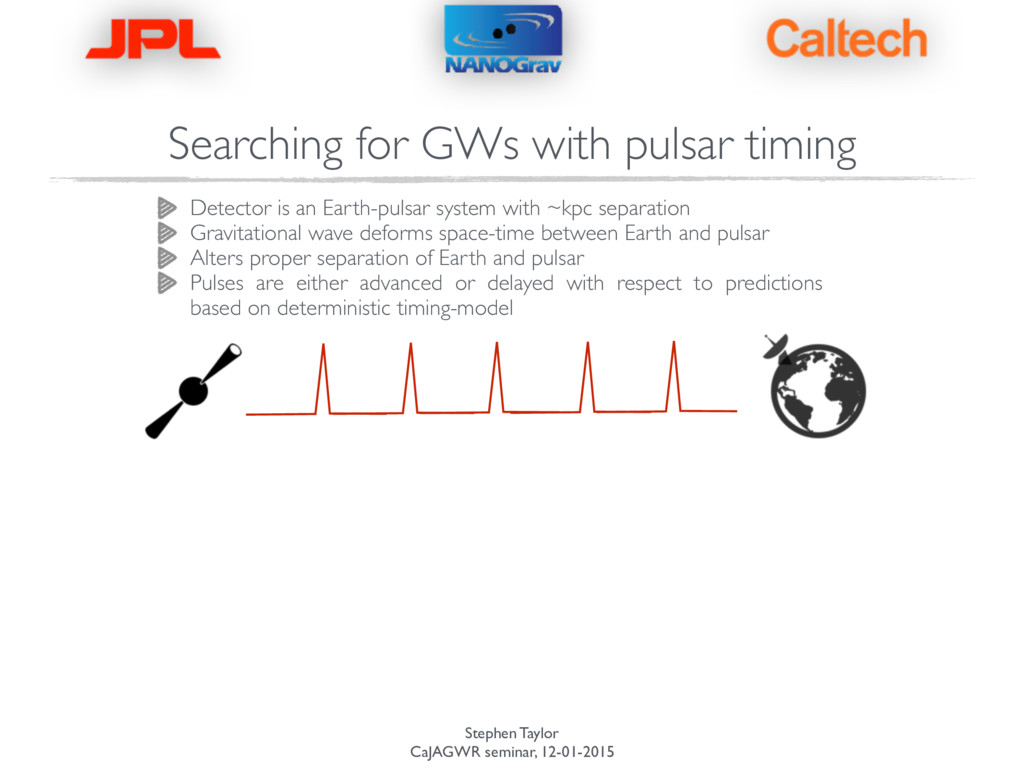
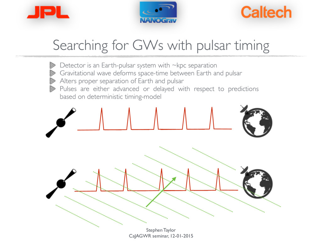
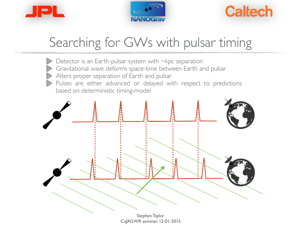
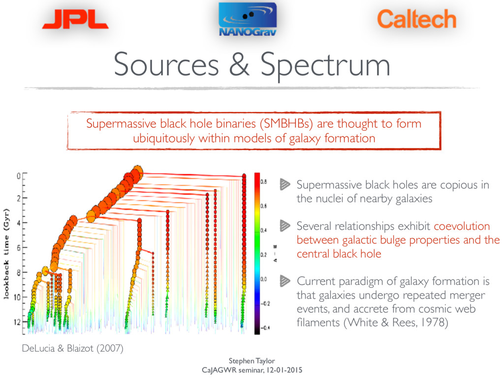
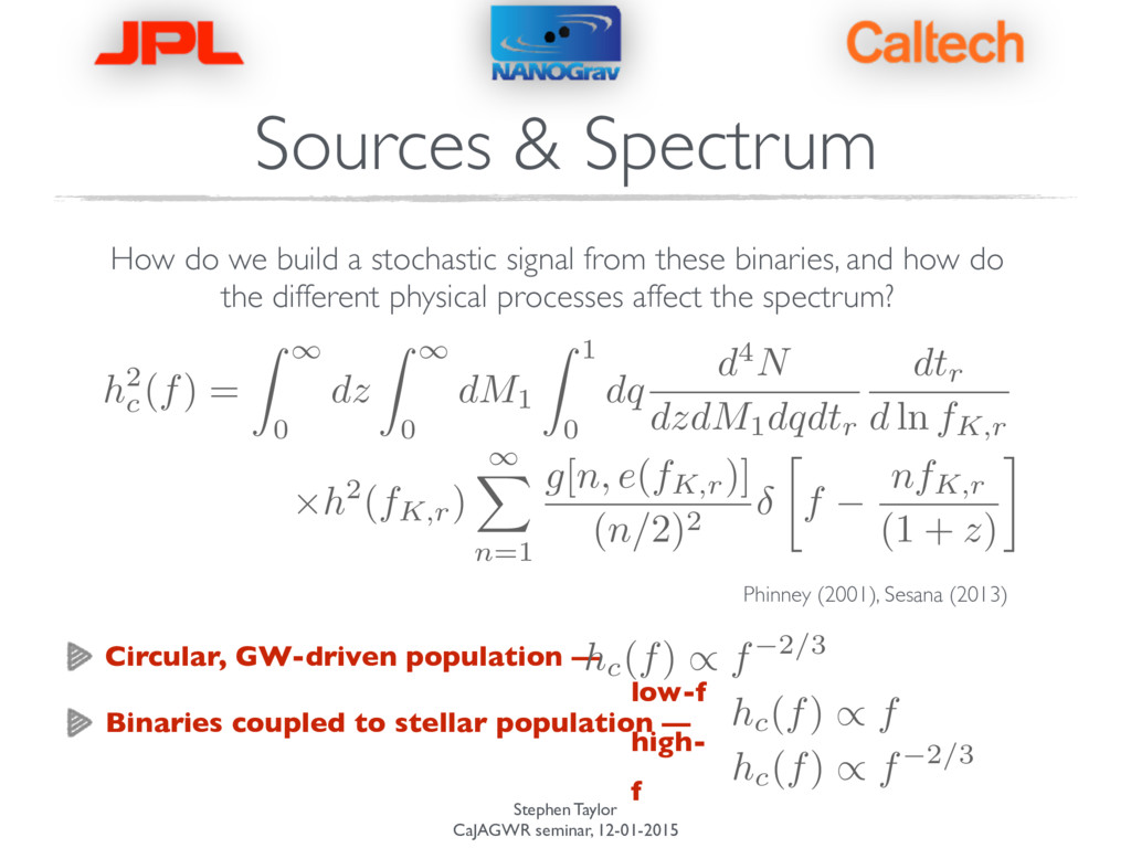
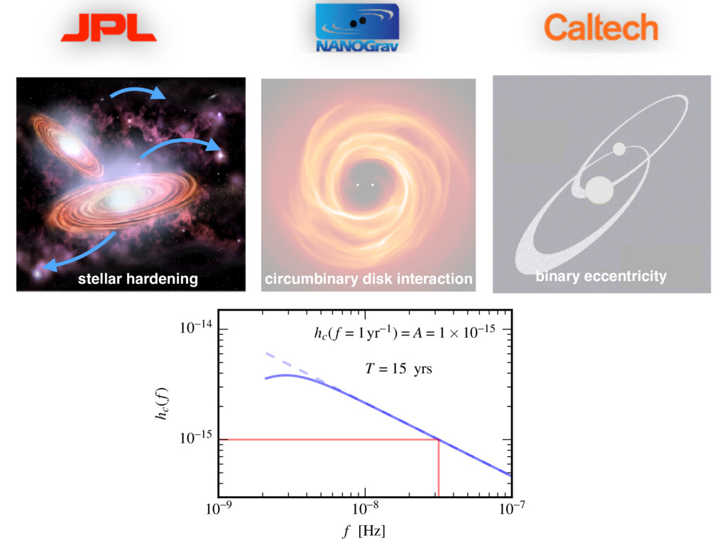
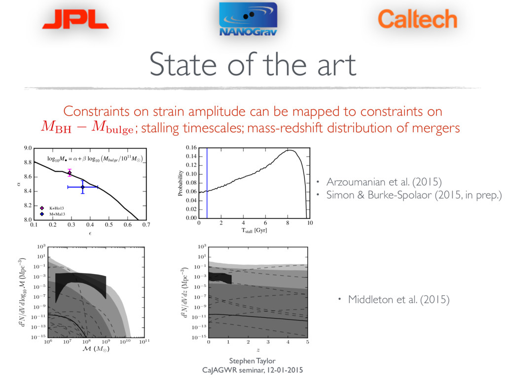
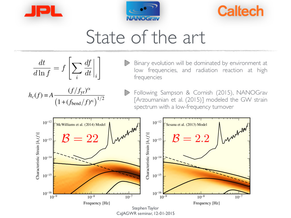
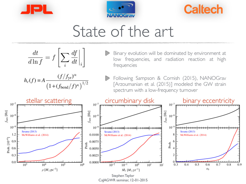
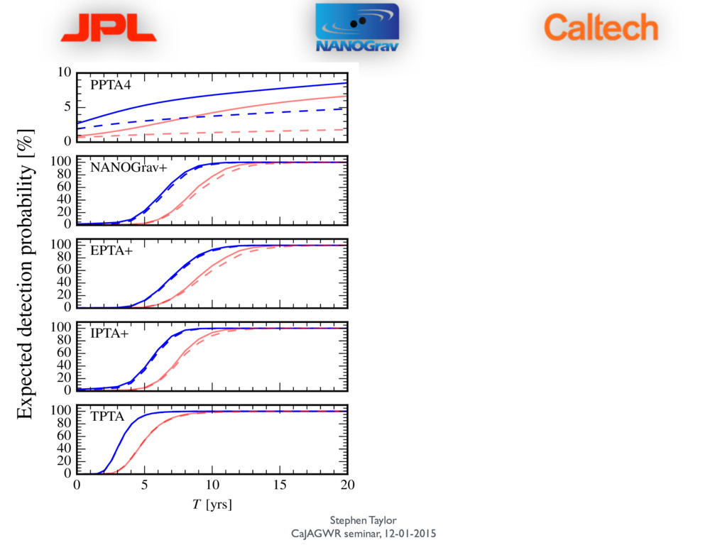
on strain amplitude can be mapped to constraints on ; stalling timescales; mass-redshift distribution of mergers MBH Mbulge ar Isotropic GWB Limit 13 0.1 0.2 0.3 0.4 0.5 0.6 0.7 ✏ 8.0 8.2 8.4 8.6 8.8 9.0 ↵ K+Ho13 M+Ma13 Figure 8. The above plot shows the translation of the 95% upper limit on Agw, Fig. 4, into the parameter space ↵-✏, which characterizes the black hole-host galaxy relation as described in Equation. (25). The parameter space above the line is inconsistent with the power-law analysis of the S13 model, as described in Simon & Burke-Spolaor (2015). Observational measurements of this parameter space are shown with errorbars. Figure 7. The above plot shows the translation of the marginalized posterior distribution of Agw, Fig. 4, into the black hole-host galaxy parameter space, which is characterized by an intercept ↵, a slope , and an intrinsic scatter ✏. Flat priors are used for ↵, , and ✏. is not informed by the distribution of Agw, while both ↵ and ✏ are, with a limit on ↵ being more strongly set. The curves show the 1, 2, and 3 contours. Relevant observational measurements are also shown, with McConnell & Ma (2013) in blue and Kormendy & Ho (2013) in magenta. Since is not strongly informed by the upper limit, we can set an upper limit in ↵-✏ space by marginalizing over . That upper limit is shown in Fig. 8. & Ho 2013; McConnell & Ma 2013, e.g.). The translation of an upper limit on Agw to the black hole- host galaxy parameter space is calculated as follows: p ↵, ,✏|PTA / Z d✓ p(✓) p(Agw (↵, ,✏,✓)|PTA), (26) where the posterior of Agw , p Agw (↵, ,✏,✓)|PTA , is the marginalized posterior distribution of Agw , which is shown in Fig. 4; Agw (↵, ,✏,✓) is the prediction of Agw calculated from models similar to S13; ✓ represents the galaxy stellar mass function and the galaxy merger rate; and p ↵, ,✏|PTA is the marginalized posterior distribution of the black hole-host galaxy relation, which is shown in Fig. 7. For this analysis, we use two leading measurements of the galaxy stellar mass function, Ilbert et al. (2013) and Tomczak et al. (2014), and two measurements of the galaxy merger rate, Robotham et al. (2014) and Keenan et al. (2014), as the basis for simulating a local population of binary SMBHs. A flat prior is used for ↵, , and ✏, and the posterior on Agw using a uniform prior, as seen in Fig. 4, is directly translated into this parameter space. The result of which is shown in Fig. 7. is clearly not informed by a PTA posterior, but the combination of ↵ and ✏ are, with the strongest limit being set on ↵. Fig. 8 shows the translation of our posterior on Agw into ↵-✏ parameter space with observational measurements of the parameters from Kormendy & Ho (2013) and McConnell & Ma (2013). Assuming a power-law analysis of the S13 model, as Figure 8. The above plot shows the translation of the 95% upper limit on Agw, Fig. 4, into the parameter space ↵-✏, which characterizes the black hole-host galaxy relation as described in Equation. (25). The parameter space above the line is inconsistent with the power-law analysis of the S13 model, as described in Simon & Burke-Spolaor (2015). Observational measurements of this parameter space are shown with errorbars. 0 2 4 6 8 10 Tstall [Gyr] 0.00 0.02 0.04 0.06 0.08 0.10 0.12 0.14 0.16 Probability Figure 9. By introducing the parameter Tstall, as described in Simon & Burke-Spolaor (2015), we can start to explore the inconsistency of our upper limit with power-law models for the GW background. In the above plot, we allow Tstall to vary while using the M• - Mbulge relation Kormendy & Ho (2013). The probability of Tstall is a direct translation of the posterior on Agw from Fig. 4. The blue line is the 95% lower limit on Tstall, which we set at 0.73 Gyr. While this is not sufficiently constraining to make meaningful astrophysical statements, this parameter may be useful for future PTA upper limits. not reach the GW-dominant regime in our assumed timescale (they “stall"); the ‘classical’ assumption of a power-law strain spectrum in the PTA band is incorrect and in fact there is a turn-over in the strain spectrum at lower frequencies (see Sec. 4.2.2); or that the measured astronomical parameters are not correct for the population of binary SMBHs in the PTA band. As the possibility for a different strain spectrum curve is discussed in Sec. 4.2.2, let us explore the potential for ‘stalling’ within the model described so far in this section. Using the galaxy merger rate density as a proxy for the black hole merger rate density implies as assumption that the events occur at a similar cosmological time. If there was signifi- cant stalling in the binary black hole population, then these events would be offset in cosmological time by some ‘stalling Astrophysics from PTAs L3 106 107 108 109 1010 1011 M (M ) 10 15 10 13 10 11 10 9 10 7 10 5 10 3 10 1 101 103 d2N/dV dlog10 M (Mpc 3) Ast 0 1 2 3 4 5 z 10 15 10 13 10 11 10 9 10 7 10 5 10 3 10 1 101 103 d2N/dV dz (Mpc 3) Figure 1. Posteriors for the merger rate density. The top row shows the merger rate density in chirp mass (integrated o 2 15 • Arzoumanian et al. (2015) • Simon & Burke-Spolaor (2015, in prep.) • Middleton et al. (2015) Figure 6. One- and two-dimensional posterior probability density plots of the spectrum model parameters Agw, fbend, and . In the one-dimensional plots, we show the posterior probability from the 9-year data set (blue), the 5-year dataset (dashed red) and the prior distribution used in both analyses (green). In the two dimensional plots we show a heat map along with the one (solid), two (dashed), and three (dash-dotted) sigma credible regions. model A is on the left and model B is on the right. (2004), McConnell & Ma (2013)) as it is the observed parameter that is most easily constrained by NANOGrav data. Specifically, we constrain the M• -Mbulge relation: log10 M• = ↵+ log10 Mbulge/1011M . (25) In addition to ↵ and , observational measurements of this relation also fit for ✏, the intrinsic scatter of individual galaxy measurements around the common ↵, trend line. In prac- tice, ↵ and ✏ have the greatest impact on predictions of Agw , and all observational measurements agree with ⇡ 1. PTAs are most sensitive to binary SMBHs where both black holes are &108M (e.g. Sesana et al. (2008)). Therefore M• -Mbulge relations that are derived including the most mas- sive systems are the most relevant to understanding the population in the PTA band. Several recent measurements of the M• -Mbulge relation specifically include high-galaxy-mass measurements, e.g. those from Brightest Cluster Galaxies (BCGs). As these fits include the high-mass black holes that we expect to dominate the PTA signals, we take these as the “gold standard" for comparison with PTA limits (Kormendy

Stephen Taylor CaJAGWR seminar, 12-01-2015 State of the art Binary
evolution will be dominated by environment at low frequencies, and radiation reaction at high frequencies dt d ln f = f " X i df dt i #

Stephen Taylor CaJAGWR seminar, 12-01-2015 State of the art t/d
ln f term) of this equation (see Colpi 2014, for a w of SMBHB coalescence). Following Sampson et al. 5) we can generalize the frequency dependence of the n spectrum to dt d ln f = f ✓ d f dt ◆-1 = f X i ✓ d f dt ◆ i !-1 , (23) e i ranges over many physical processes that are driv- he binary to coalescence. If we restrict this sum to GW- n evolution and an unspeciﬁed physical process then the n spectrum is now hc (f) = A (f/fyr )↵ 1+(fbend/f) 1/2 , (24) Binary evolution will be dominated by environment at low frequencies, and radiation reaction at high frequencies dt d ln f = f " X i df dt i # Following Sampson & Cornish (2015), NANOGrav [Arzoumanian et al. (2015)] modeled the GW strain spectrum with a low-frequency turnover

ln f term) of this equation (see Colpi 2014, for a w of SMBHB coalescence). Following Sampson et al. 5) we can generalize the frequency dependence of the n spectrum to dt d ln f = f ✓ d f dt ◆-1 = f X i ✓ d f dt ◆ i !-1 , (23) e i ranges over many physical processes that are driv- he binary to coalescence. If we restrict this sum to GW- n evolution and an unspeciﬁed physical process then the n spectrum is now hc (f) = A (f/fyr )↵ 1+(fbend/f) 1/2 , (24) Binary evolution will be dominated by environment at low frequencies, and radiation reaction at high frequencies dt d ln f = f " X i df dt i # 12 10-9 10-8 10-7 Frequency [Hz] 10-16 10-15 10-14 10-13 10-12 Characteristic Strain [hc(f)] McWilliams et al. (2014) Model 10-9 10-8 10-7 Frequency [Hz] 10-16 10-15 10-14 10-13 10-12 Characteristic Strain [hc(f)] Sesana et al. (2013) Model Figure 5. Probability density plots of the recovered GWB spectra for models A and B using the broken-power-law model parameterized by (Agw, fbend, and ) Following Sampson & Cornish (2015), NANOGrav [Arzoumanian et al. (2015)] modeled the GW strain spectrum with a low-frequency turnover B = 22 B = 2.2

ln f term) of this equation (see Colpi 2014, for a w of SMBHB coalescence). Following Sampson et al. 5) we can generalize the frequency dependence of the n spectrum to dt d ln f = f ✓ d f dt ◆-1 = f X i ✓ d f dt ◆ i !-1 , (23) e i ranges over many physical processes that are driv- he binary to coalescence. If we restrict this sum to GW- n evolution and an unspeciﬁed physical process then the n spectrum is now hc (f) = A (f/fyr )↵ 1+(fbend/f) 1/2 , (24) Binary evolution will be dominated by environment at low frequencies, and radiation reaction at high frequencies dt d ln f = f " X i df dt i # Following Sampson & Cornish (2015), NANOGrav [Arzoumanian et al. (2015)] modeled the GW strain spectrum with a low-frequency turnover 16 10-9 10-8 10-7 fturn [Hz] 103 104 105 106 ⇢ [M pc-3] 0.0 0.3 0.6 0.9 1.2 Prob. [10-6] Sesana (2013) McWilliams et al. (2014) Figure 10. (top): Empirical mapping from fturn to ⇢ (left) and ˙ M1 (right). (bottom): Posterior distributions for the mass density of stars in the galactic core 10-9 10-8 10-7 fturn [Hz] 10-2 10-1 100 101 102 ˙ M1 [M yr-1] 0.0000 0.0025 0.0050 0.0075 0.0100 Prob. Sesana (2013) McWilliams et al. (2014) 10. (top): Empirical mapping from fturn to ⇢ (left) and ˙ M1 (right). (bottom): Posterior distributions for the mass density of stars in the galactic core 16 Figure 10. (top): Empirical mapping from fturn to ⇢ (left) and ˙ M1 (right). (bottom): Posterior distributions for the mass density of stars in the galactic core (left) and the accretion rate of the primary black hole from a circumbinary disk (right). These distributions are constructed by ﬁrst converting the marginalized distribution of fbend to a distribution of fturn via Eq. (30), and then using the empirical mapping described in the text to convert from fturn to the astrophysical quantities ⇢ and ˙ M1, respectively. raise the stellar mass density to match a corresponding increase in binary mass so that the transition frequency is main- tained. Furthermore, modeling the distribution of black holes masses in Eq. (35) without the lognormal component or redshift evolution will increase the contribution of lower mass binaries to the GW strain budget, leading to smaller stellar mass density constraints than reported in Fig. 10. Varying the normalization, a, and exponent, b, of the M - relation such that a 2 [7,9] and b 2 [4,6] has very little impact on the environmental constraints. 5.1.3. Constraints on SMBH binary population eccentricity It is not only the astrophysical environment of SMBH binaries that can induce a bend in the characteristic strain spectrum. Binaries with non-zero eccentricity emit GWs at a spectrum of harmonics of the orbital frequency. The cumulative effect over the entire population can lead to a depletion of the low frequency strain spectrum (Enoki et al. 2007; Sesana 2013; Ravi et al. 2014; Huerta et al. 2015), and a turnover whose shape can be captured with the parametrized spectrum model employed in this paper. Hence, we can use our fturn posterior from the marginalization of fbend over all  to de- duce constraints on the eccentricity of binaries at some refer- 10-9 10-8 10-7 fturn [Hz] 0.3 0.4 0.5 0.6 0.7 0.8 0.9 e0 0 2 4 6 8 Prob. Sesana (2013) McWilliams et al. (2014) Figure 11. Same as Figure 10 except now we display the empirical mapping (top) and posterior distribution (bottom) for the eccentricity of SMBH stellar scattering circumbinary disk binary eccentricity

Stephen Taylor CaJAGWR seminar, 12-01-2015 Observational strategy changes advocated in
Shannon et al. (2015) [4 pulsars, A<1e-15] State of the art

Stephen Taylor CaJAGWR seminar, 12-01-2015 High-cadence campaign to detect GW
background at to combat depletion of low-frequency signal due to environmental couplings. If the spectrum is just a power-law with a lower overall amplitude (binary stalling) then ﬁrst evidence for GW background will show up as timing noise in PSR J1909-3744 when longer data spans are achieved. Observational strategy changes advocated in Shannon et al. (2015) [4 pulsars, A<1e-15] f & 6 nHz State of the art

Stephen Taylor CaJAGWR seminar, 12-01-2015 Detection of the GW background
has different demands from placing tight upper limits. The smoking-gun is the “Hellings and Downs curve” — the overlap reduction function for an isotropic stochastic background. Background detection statistic uses cross-correlations between pulsar pairs. Requires many pulsars to synthesize pairings for adequate measurement. So, we need many pulsars for detection! Only need a few exquisitely timed pulsars for upper limits. Detection prospects

Stephen Taylor CaJAGWR seminar, 12-01-2015 Detection prospects 0 20 40
60 80 100 120 140 160 180 pulsar angular separation [deg] -0.2 0.0 0.2 0.4 0.6 0.8 1.0 arrival time correlation N = 1 Npairs = N(N 1)/2

60 80 100 120 140 160 180 pulsar angular separation [deg] -0.2 0.0 0.2 0.4 0.6 0.8 1.0 arrival time correlation N = 1 0 20 40 60 80 100 120 140 160 180 pulsar angular separation [deg] -0.2 0.0 0.2 0.4 0.6 0.8 1.0 arrival time correlation N = 4 Npairs = N(N 1)/2

60 80 100 120 140 160 180 pulsar angular separation [deg] -0.2 0.0 0.2 0.4 0.6 0.8 1.0 arrival time correlation N = 1 0 20 40 60 80 100 120 140 160 180 pulsar angular separation [deg] -0.2 0.0 0.2 0.4 0.6 0.8 1.0 arrival time correlation N = 4 0 20 40 60 80 100 120 140 160 180 pulsar angular separation [deg] -0.2 0.0 0.2 0.4 0.6 0.8 1.0 arrival time correlation N = 10 Npairs = N(N 1)/2

60 80 100 120 140 160 180 pulsar angular separation [deg] -0.2 0.0 0.2 0.4 0.6 0.8 1.0 arrival time correlation N = 1 0 20 40 60 80 100 120 140 160 180 pulsar angular separation [deg] -0.2 0.0 0.2 0.4 0.6 0.8 1.0 arrival time correlation N = 4 0 20 40 60 80 100 120 140 160 180 pulsar angular separation [deg] -0.2 0.0 0.2 0.4 0.6 0.8 1.0 arrival time correlation N = 10 0 20 40 60 80 100 120 140 160 180 pulsar angular separation [deg] -0.2 0.0 0.2 0.4 0.6 0.8 1.0 arrival time correlation N = 30 Npairs = N(N 1)/2

60 80 100 120 140 160 180 pulsar angular separation [deg] -0.2 0.0 0.2 0.4 0.6 0.8 1.0 arrival time correlation N = 1 0 20 40 60 80 100 120 140 160 180 pulsar angular separation [deg] -0.2 0.0 0.2 0.4 0.6 0.8 1.0 arrival time correlation N = 4 0 20 40 60 80 100 120 140 160 180 pulsar angular separation [deg] -0.2 0.0 0.2 0.4 0.6 0.8 1.0 arrival time correlation N = 10 0 20 40 60 80 100 120 140 160 180 pulsar angular separation [deg] -0.2 0.0 0.2 0.4 0.6 0.8 1.0 arrival time correlation N = 30 0 20 40 60 80 100 120 140 160 180 pulsar angular separation [deg] -0.2 0.0 0.2 0.4 0.6 0.8 1.0 arrival time correlation N = 50 Npairs = N(N 1)/2

Stephen Taylor CaJAGWR seminar, 12-01-2015 Compute detection probability (DP) in
terms of true background signal and time. We don’t know what the true amplitude is. Compute Average the DP over this. We now have expected DP as function of time Detection prospects p(Atrue |Aul)

Stephen Taylor CaJAGWR seminar, 12-01-2015 0.0 0.5 1.0 1.5 2.0
2.5 3.0 3.5 4.0 p(Atrue |Aul) ⇥1015 PPTA p(Atrue) = {Sesana (2013), fstall = 0.0} p(Atrue) = {Sesana (2013), fstall = 0.9} 0.0 0.5 1.0 1.5 2.0 Atrue ⇥10-15 0.0 0.5 1.0 1.5 2.0 2.5 3.0 3.5 4.0 p(Atrue |Aul) ⇥1015 NANOGrav p(Atrue) = {Sesana (2013), fstall = 0.0} p(Atrue) = {Sesana (2013), fstall = 0.9} Detection prospects Update prior [Sesana (2013)] with tighter constraints from PPTA [Shannon et al. (2015)] Can do same for NANOGrav, but PPTA limit is stronger

Stephen Taylor CaJAGWR seminar, 12-01-2015 Upper limits achievable with only
a few exquisitely timed pulsars. This array conﬁguration is sub-optimal for GWB detection. Timing many pulsars allows the quadrupolar spatial correlation signature of the GWB to be sampled at many different angular separations. Regularly adding more pulsars to our arrays will continually improve our detection prospects on top of the gains we already make by timing existing pulsars for longer. This helps mitigate the deleterious inﬂuences of binary stalling and environmental couplings, such that high detection probabilities are delayed by only a few years. 0 5 10 PPTA4 0 20 40 60 80 100 NANOGrav+ 0 20 40 60 80 100 EPTA+ 0 20 40 60 80 100 IPTA+ 0 5 10 15 20 T [yrs] 0 20 40 60 80 100 TPTA Expected detection probability [%]

Stephen Taylor CaJAGWR seminar, 12-01-2015 Stephen Taylor CaJAGWR seminar, 12-01-2015
0 5 10 PPTA4 0 20 40 60 80 100 NANOGrav+ 0 20 40 60 80 100 EPTA+ 0 20 40 60 80 100 IPTA+ 0 5 10 15 20 T [yrs] 0 20 40 60 80 100 TPTA Expected detection probability [%]

Stephen Taylor CaJAGWR seminar, 12-01-2015 10-9 10-8 10-7 f [Hz]
10-15 10-14 hc( f) hc(f = 1yr-1) = A = 1⇥10-15 T = 9 yrs 10-9 10-8 10-7 f [Hz] 10-12 10-11 10-10 10-9 10-8 10-7 10-6 10-5 10-4 10-3 Sh(f) [s3] Sh( f) = hc( f)2/(12⇡2 f3) T = 9 yrs Stephen Taylor CaJAGWR seminar, 12-01-2015 0 5 10 PPTA4 0 20 40 60 80 100 NANOGrav+ 0 20 40 60 80 100 EPTA+ 0 20 40 60 80 100 IPTA+ 0 5 10 15 20 T [yrs] 0 20 40 60 80 100 TPTA Expected detection probability [%]

10-15 10-14 hc( f) hc(f = 1yr-1) = A = 1⇥10-15 T = 9 yrs 10-9 10-8 10-7 f [Hz] 10-15 10-14 hc(f) hc( f = 1yr-1) = A = 1⇥10-15 T = 11 yrs 10-9 10-8 10-7 f [Hz] 10-12 10-11 10-10 10-9 10-8 10-7 10-6 10-5 10-4 10-3 Sh(f) [s3] Sh( f) = hc( f)2/(12⇡2 f3) T = 9 yrs 10-9 10-8 10-7 f [Hz] 10-12 10-11 10-10 10-9 10-8 10-7 10-6 10-5 10-4 10-3 Sh(f) [s3] Sh( f) = hc( f)2/(12⇡2 f3) T = 11 yrs Stephen Taylor CaJAGWR seminar, 12-01-2015 0 5 10 PPTA4 0 20 40 60 80 100 NANOGrav+ 0 20 40 60 80 100 EPTA+ 0 20 40 60 80 100 IPTA+ 0 5 10 15 20 T [yrs] 0 20 40 60 80 100 TPTA Expected detection probability [%]

10-15 10-14 hc( f) hc(f = 1yr-1) = A = 1⇥10-15 T = 9 yrs 10-9 10-8 10-7 f [Hz] 10-15 10-14 hc(f) hc( f = 1yr-1) = A = 1⇥10-15 T = 11 yrs 10-9 10-8 10-7 f [Hz] 10-15 10-14 hc( f) hc(f = 1yr-1) = A = 1⇥10-15 T = 15 yrs 10-9 10-8 10-7 f [Hz] 10-12 10-11 10-10 10-9 10-8 10-7 10-6 10-5 10-4 10-3 Sh(f) [s3] Sh( f) = hc( f)2/(12⇡2 f3) T = 9 yrs 10-9 10-8 10-7 f [Hz] 10-12 10-11 10-10 10-9 10-8 10-7 10-6 10-5 10-4 10-3 Sh(f) [s3] Sh( f) = hc( f)2/(12⇡2 f3) T = 11 yrs 10-9 10-8 10-7 f [Hz] 10-12 10-11 10-10 10-9 10-8 10-7 10-6 10-5 10-4 10-3 Sh(f) [s3] Sh( f) = hc( f)2/(12⇡2 f3) T = 15 yrs Stephen Taylor CaJAGWR seminar, 12-01-2015 0 5 10 PPTA4 0 20 40 60 80 100 NANOGrav+ 0 20 40 60 80 100 EPTA+ 0 20 40 60 80 100 IPTA+ 0 5 10 15 20 T [yrs] 0 20 40 60 80 100 TPTA Expected detection probability [%]

10-15 10-14 hc( f) hc(f = 1yr-1) = A = 1⇥10-15 T = 9 yrs 10-9 10-8 10-7 f [Hz] 10-15 10-14 hc(f) hc( f = 1yr-1) = A = 1⇥10-15 T = 11 yrs 10-9 10-8 10-7 f [Hz] 10-15 10-14 hc( f) hc(f = 1yr-1) = A = 1⇥10-15 T = 15 yrs 10-9 10-8 10-7 f [Hz] 10-15 10-14 hc( f) hc(f = 1yr-1) = A = 1⇥10-15 T = 30 yrs 10-9 10-8 10-7 f [Hz] 10-12 10-11 10-10 10-9 10-8 10-7 10-6 10-5 10-4 10-3 Sh(f) [s3] Sh( f) = hc( f)2/(12⇡2 f3) T = 9 yrs 10-9 10-8 10-7 f [Hz] 10-12 10-11 10-10 10-9 10-8 10-7 10-6 10-5 10-4 10-3 Sh(f) [s3] Sh( f) = hc( f)2/(12⇡2 f3) T = 11 yrs 10-9 10-8 10-7 f [Hz] 10-12 10-11 10-10 10-9 10-8 10-7 10-6 10-5 10-4 10-3 Sh(f) [s3] Sh( f) = hc( f)2/(12⇡2 f3) T = 15 yrs 10-9 10-8 10-7 f [Hz] 10-12 10-11 10-10 10-9 10-8 10-7 10-6 10-5 10-4 10-3 Sh(f) [s3] Sh( f) = hc( f)2/(12⇡2 f3) T = 30 yrs Stephen Taylor CaJAGWR seminar, 12-01-2015 0 5 10 PPTA4 0 20 40 60 80 100 NANOGrav+ 0 20 40 60 80 100 EPTA+ 0 20 40 60 80 100 IPTA+ 0 5 10 15 20 T [yrs] 0 20 40 60 80 100 TPTA Expected detection probability [%]

Stephen Taylor CaJAGWR seminar, 12-01-2015 Requirements of upper limits versus
detection very different. We need many pulsars for detection. Binary stalling or ﬁnal-parsec processes may diminish low-frequency signal, but the effect is not severe since we continually expand our pulsar catalogs. We have a ~80% probability of background detection within 10 years, even in pessimistic scenarios. Detection prospects

Stephen Taylor CaJAGWR seminar, 12-01-2015 D N 16, 2015 Preprint
typeset using L A TEX style emulateapj v. 12/16/11 ARE WE THERE YET? TIME TO DETECTION OF NANOHERTZ GRAVITATIONAL WAVES BASED ON PULSAR-TIMING ARRAY LIMITS S. R. T 1,2?, M. V 1,2, J. A. E 1,2,†, C. M. F. M 2, 3, 1, T. J. W. L 1,2, & R. H 1,2,† Draft version November 16, 2015 ABSTRACT Decade-long timing observations of arrays of millisecond pulsars have placed highly constraining upper limits on the amplitude of the nanohertz gravitational-wave stochastic signal from the mergers of supermassive black- hole binaries (⇠ 10-15 strain at f = 1/yr). These limits suggest that binary merger rates have been overestimated, or that environmental influences from nuclear gas or stars accelerate orbital decay, reducing the gravitational- wave signal at the lowest, most sensitive frequencies. This prompts the question whether nanohertz gravitational waves are likely to be detected in the near future. In this letter, we answer this question quantitatively using simple statistical estimates, deriving the range of true signal amplitudes that are compatible with current upper limits, and computing expected detection probabilities as a function of observation time. We conclude that small arrays consisting of the pulsars with the least timing noise, which yield the tightest upper limits, have discouraging prospects of making a detection in the next two decades. By contrast, we find large arrays are crucial to detection because the quadrupolar spatial correlations induced by gravitational waves can be well sampled by many pulsar pairs. Indeed, timing programs which monitor a large and expanding set of pulsars have an ⇠ 80% probability of detecting gravitational waves within the next ten years, under assumptions on merger rates and environmental influences ranging from optimistic to conservative. Even in the extreme case where 90% of binaries stall before merger and environmental coupling e ects diminish low-frequency gravitational-wave power, detection is delayed by at most a few years. Keywords: methods: data analysis — gravitational waves — pulsars: individual — pulsars: general 1. INTRODUCTION For the last ten years, three international collaborations have been collecting precise timing observations of the most stable 2015) imply AGW . 10-15 at 95% confidence. These limits ap- pear in tension with theoretical expectations, so much so that it seems plausible that environmental e ects in galactic centers Detection prospects

Stephen Taylor CaJAGWR seminar, 12-01-2015 Pulsar-timing arrays can detect nHz
gravitational waves and probe galactic astrophysics Current constraints in tension with basic models of SMBHB evolution Probe BH-galaxy relationships, and investigate ﬁnal- parsec astrophysics via the shape of the GW strain spectrum The GW signal may be lower than previously thought, or diminished at lower frequencies by environmental processes Large and expanding pulsar catalogs offer ~80% detection probability after a further 10 years of observations Pessimistic signal levels only delay detection by ~2-3 years. Summary

Prospects For Near-future Detection & Astrophysical Inference With Pulsar-timing Arrays

Prospects For Near-future Detection & Astrophysical Inference With Pulsar-timing Arrays

More Decks by Dr. Stephen R. Taylor

Other Decks in Science

Featured

Transcript