4/16
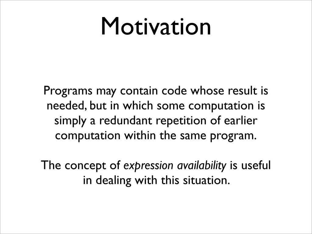
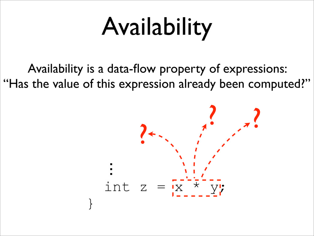
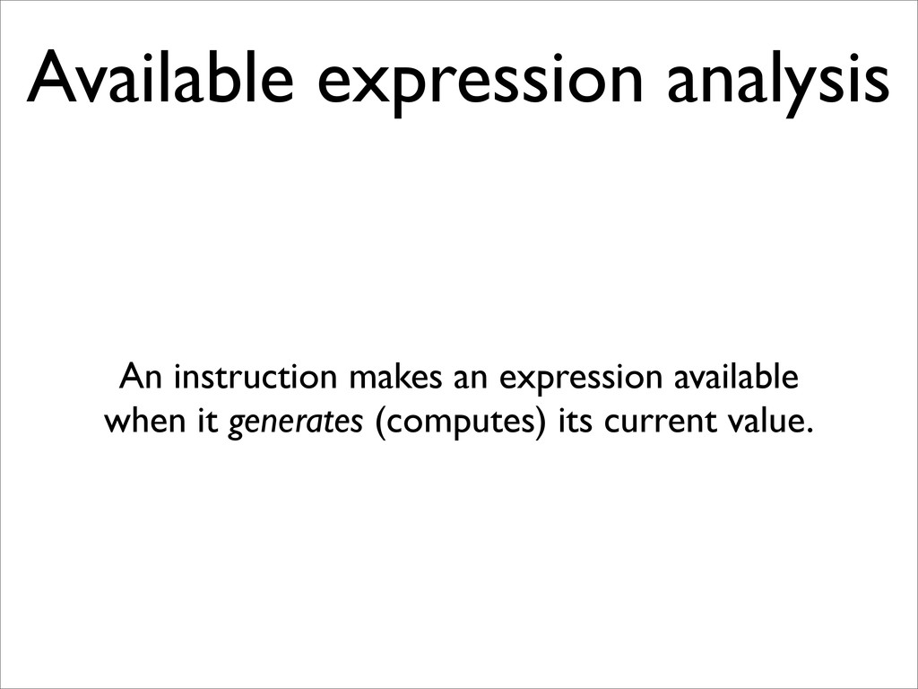
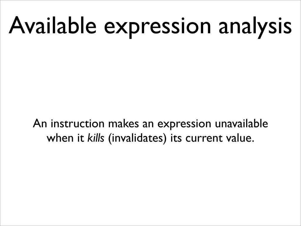
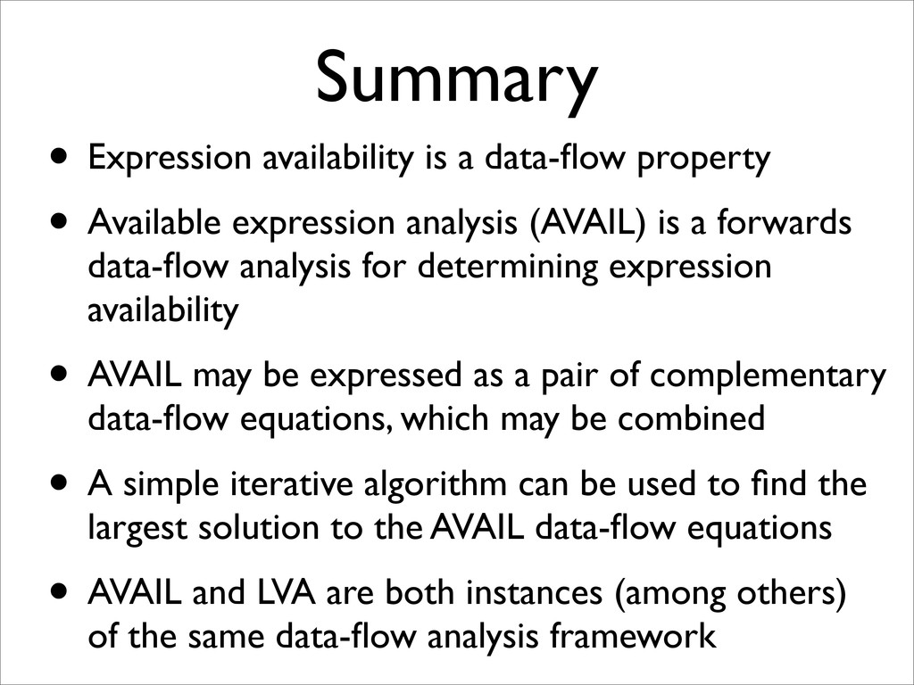
* Expression availability is a data-flow property
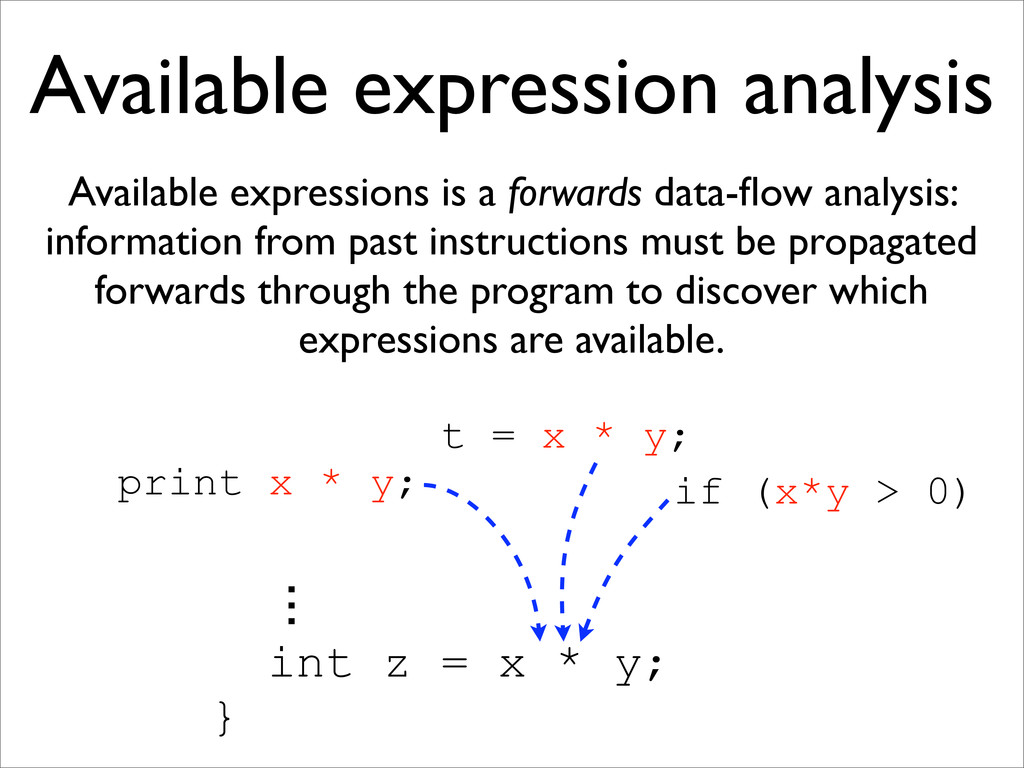
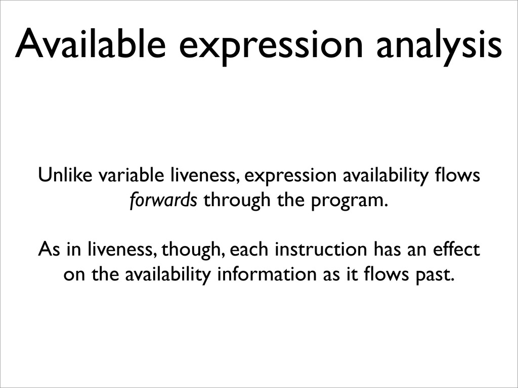
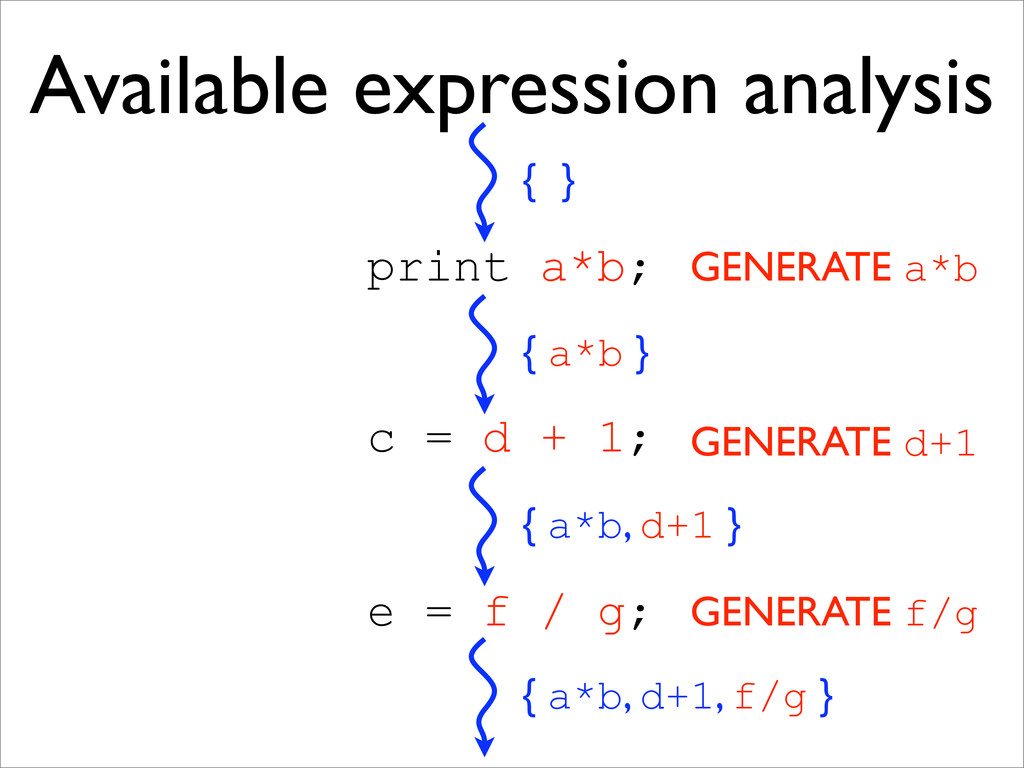
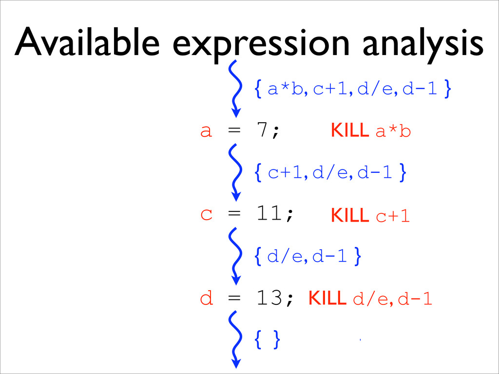
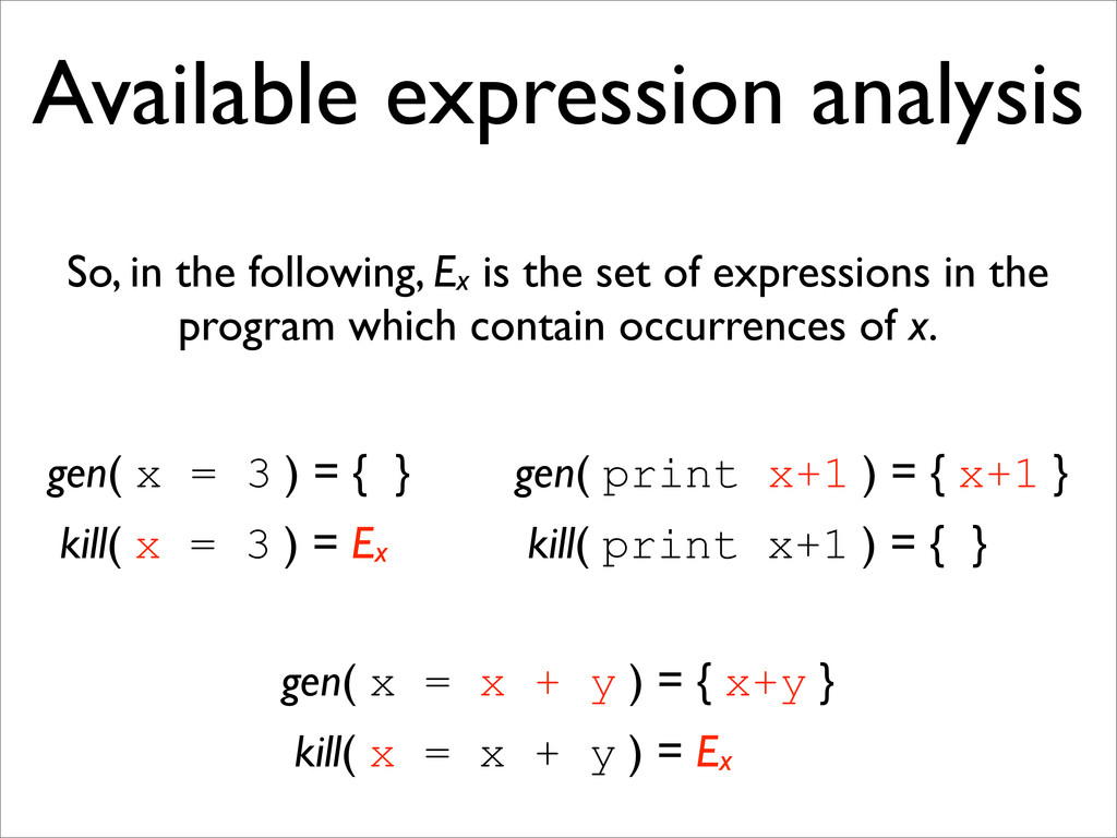
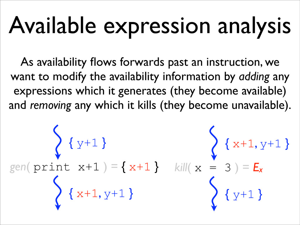
* Available expression analysis (AVAIL) is a forwards data-flow analysis for determining expression availability
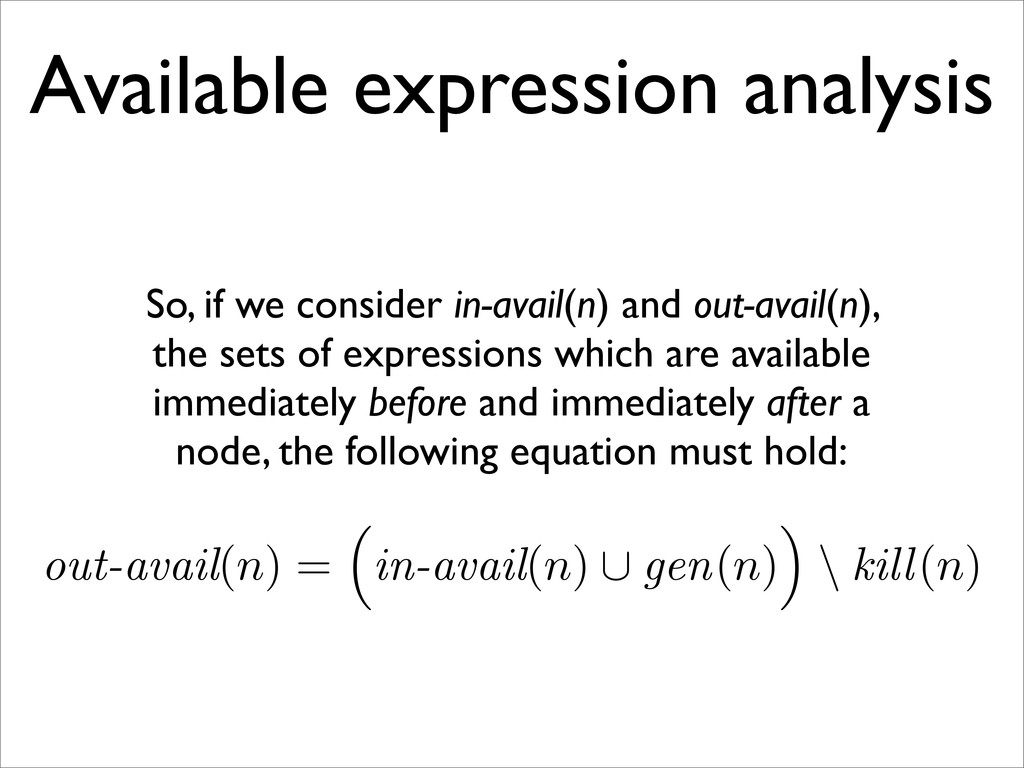
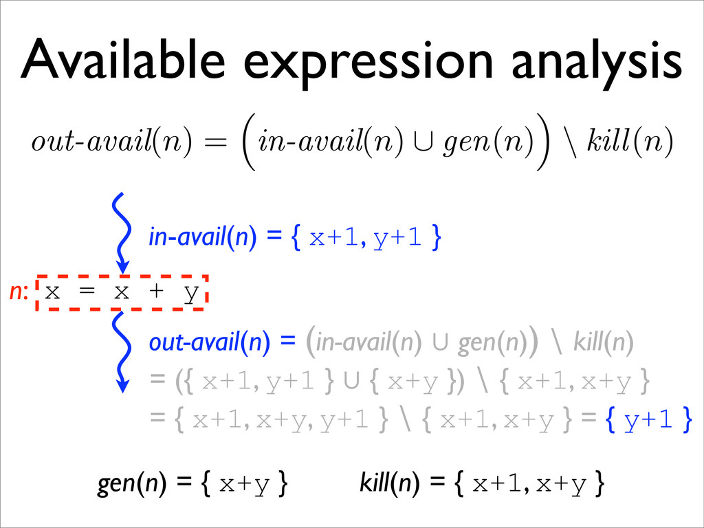
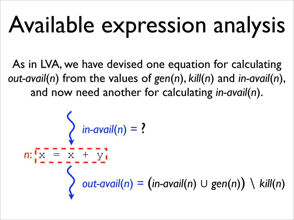
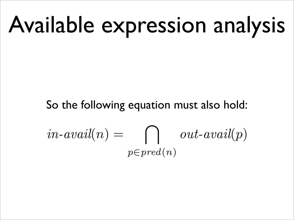
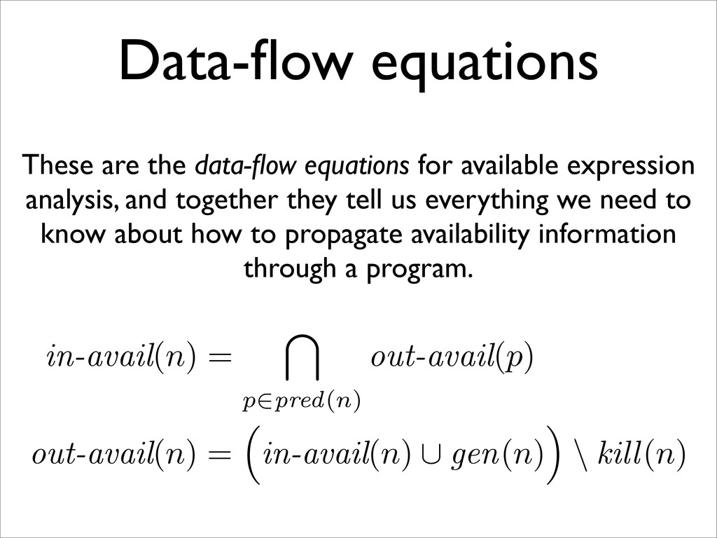
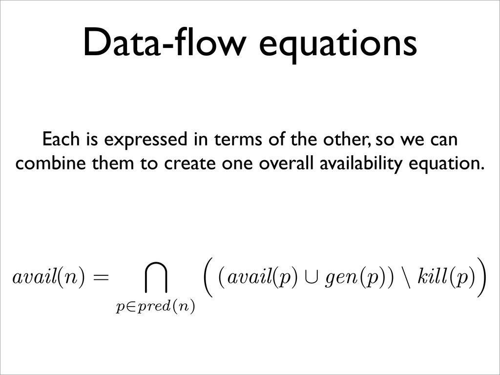
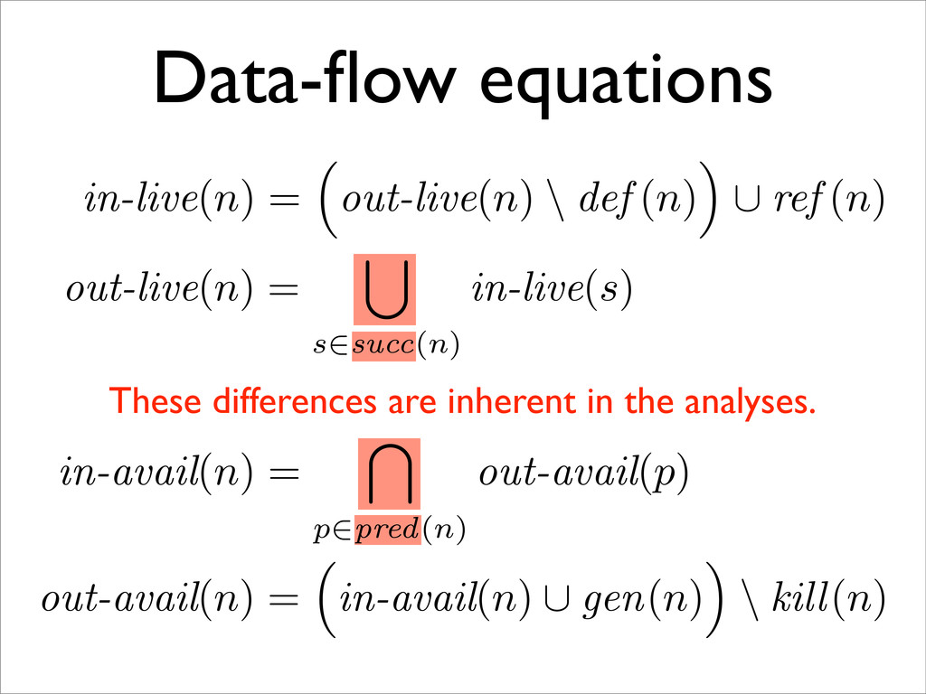
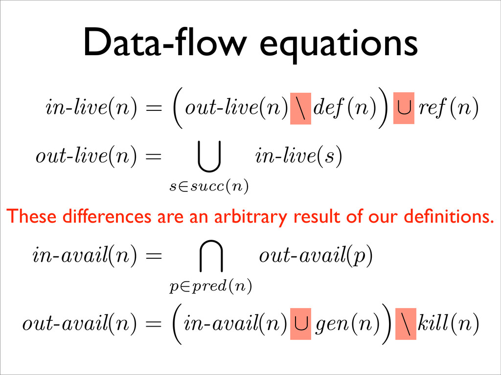
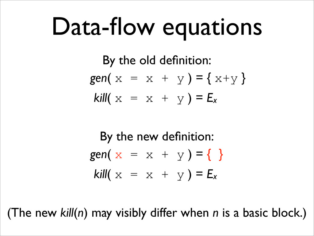
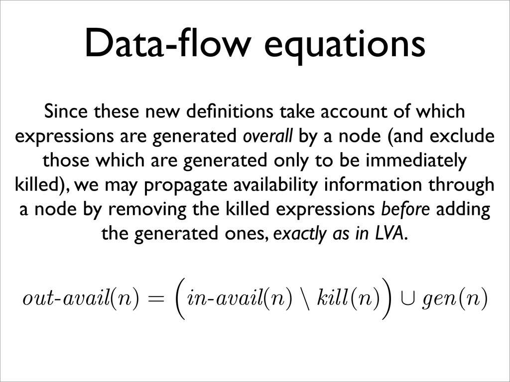
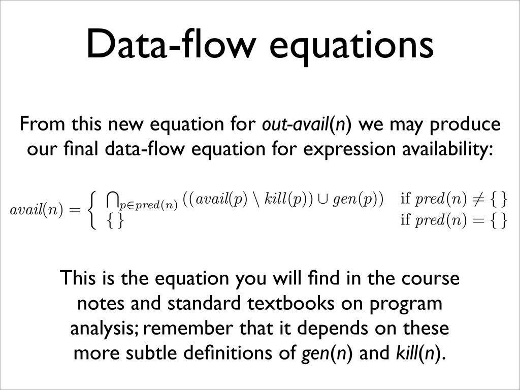
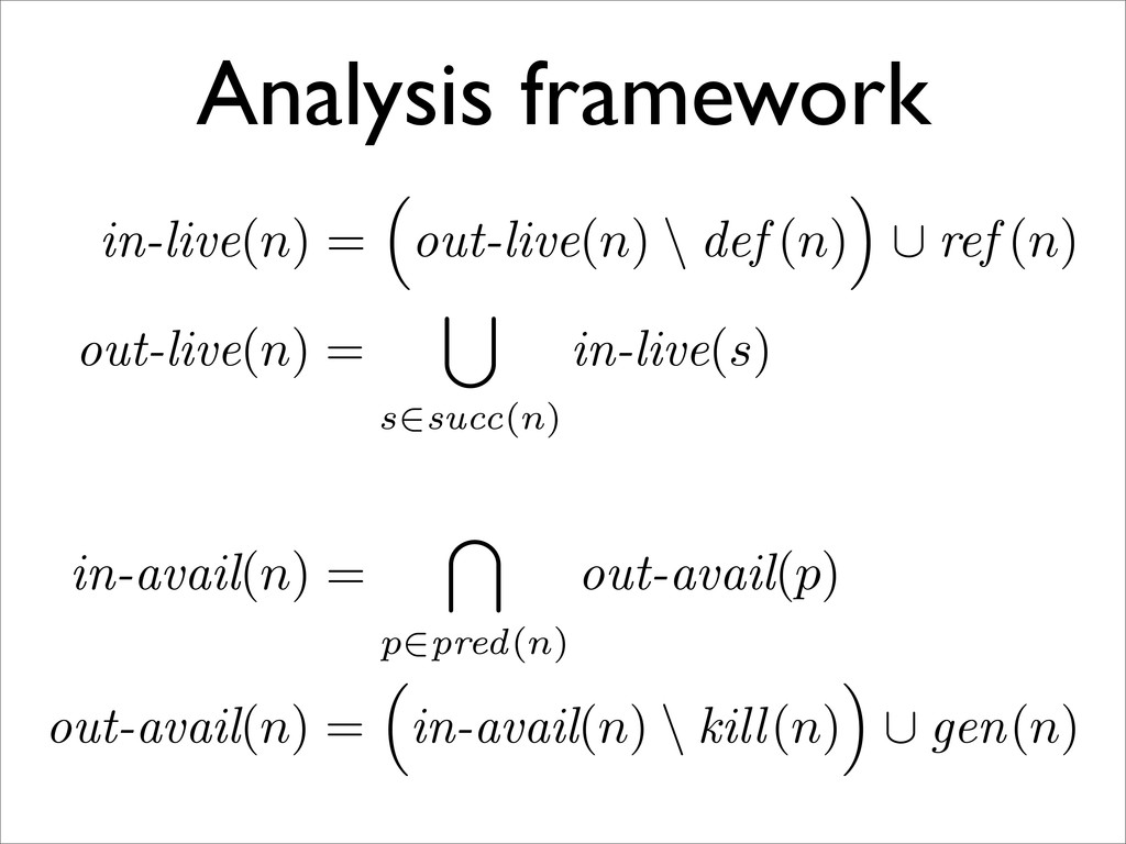
* AVAIL may be expressed as a pair of complementary data-flow equations, which may be combined
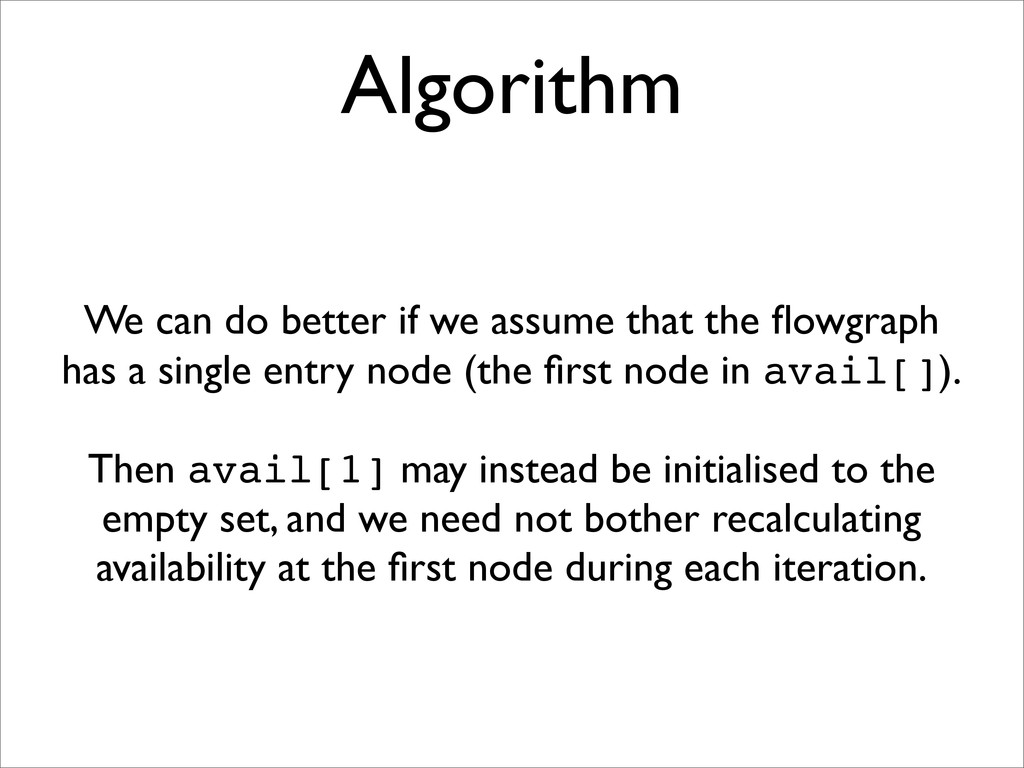
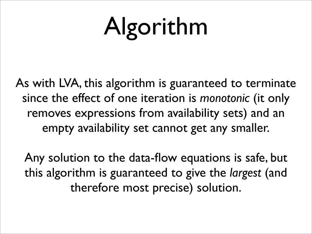
* A simple iterative algorithm can be used to find the largest solution to the AVAIL data-flow equations
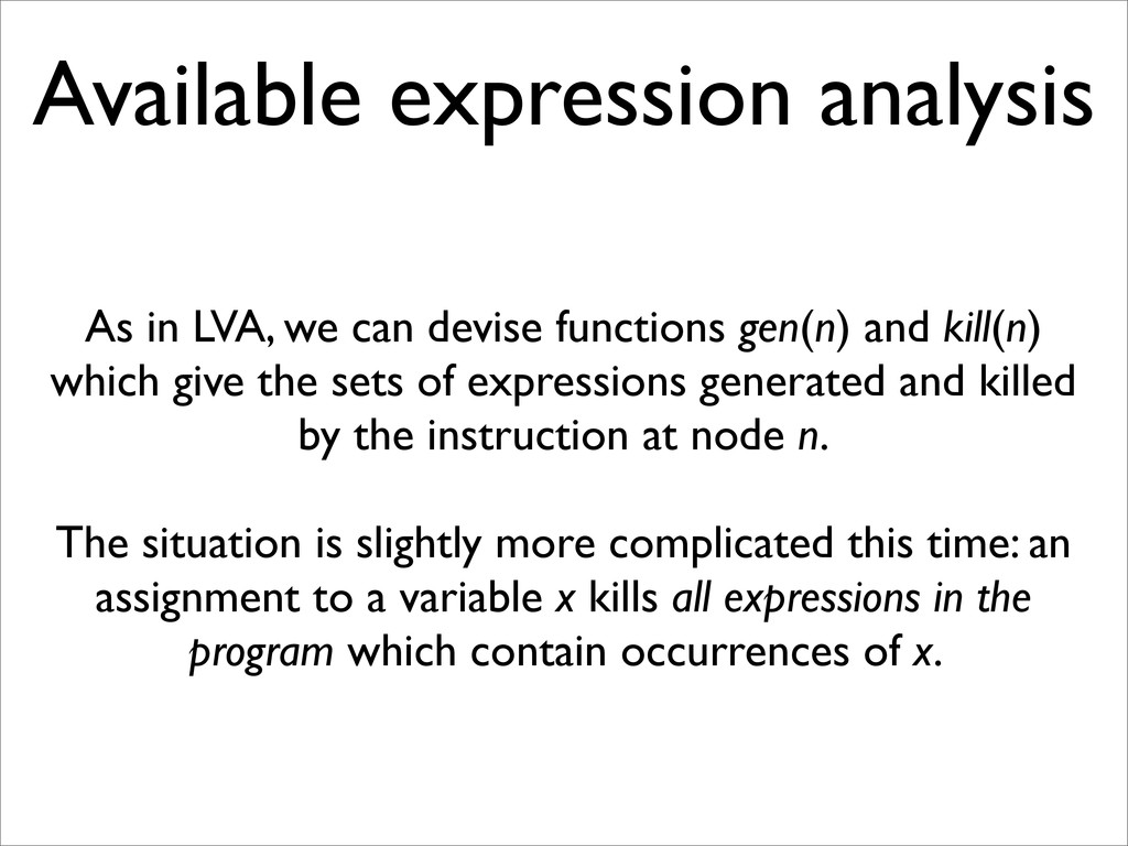
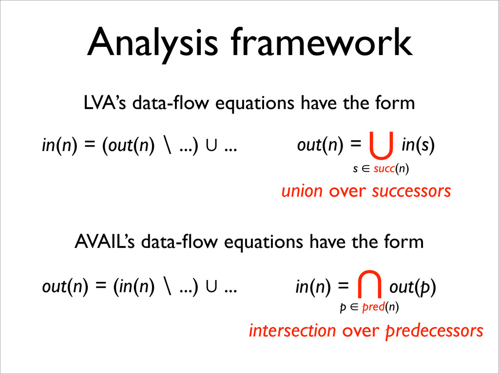
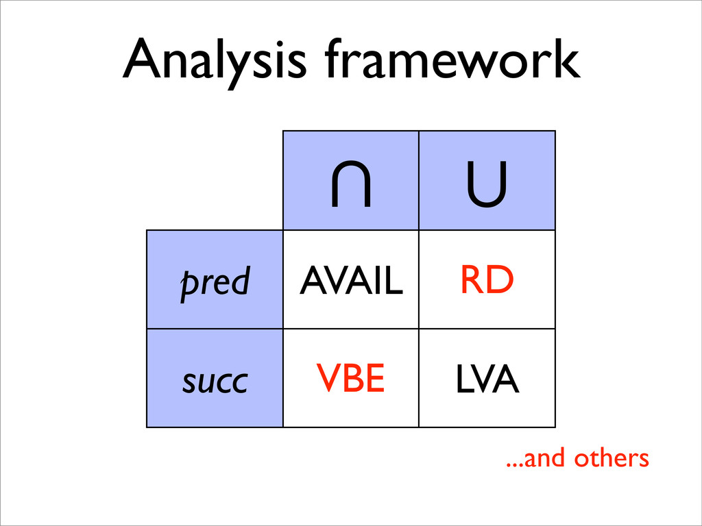
* AVAIL and LVA are both instances (among others) of the same data-flow analysis framework
![Algorithm • We again use an array, avail[], to store](https://files.speakerdeck.com/presentations/4ea51e7515006a005100a3e4/slide_44.jpg)
![Algorithm for i = 1 to n do avail[i] :=](https://files.speakerdeck.com/presentations/4ea51e7515006a005100a3e4/slide_45.jpg)
![Algorithm avail[1] := {} for i = 2 to n](https://files.speakerdeck.com/presentations/4ea51e7515006a005100a3e4/slide_47.jpg)