Multi-Date Land-Cover Mapping with NAIP Imagery - Arkansas 2006-2010 by Bruce Gorham

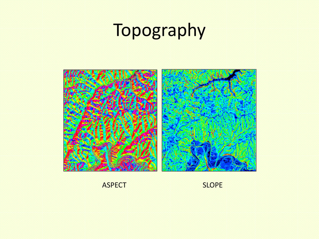
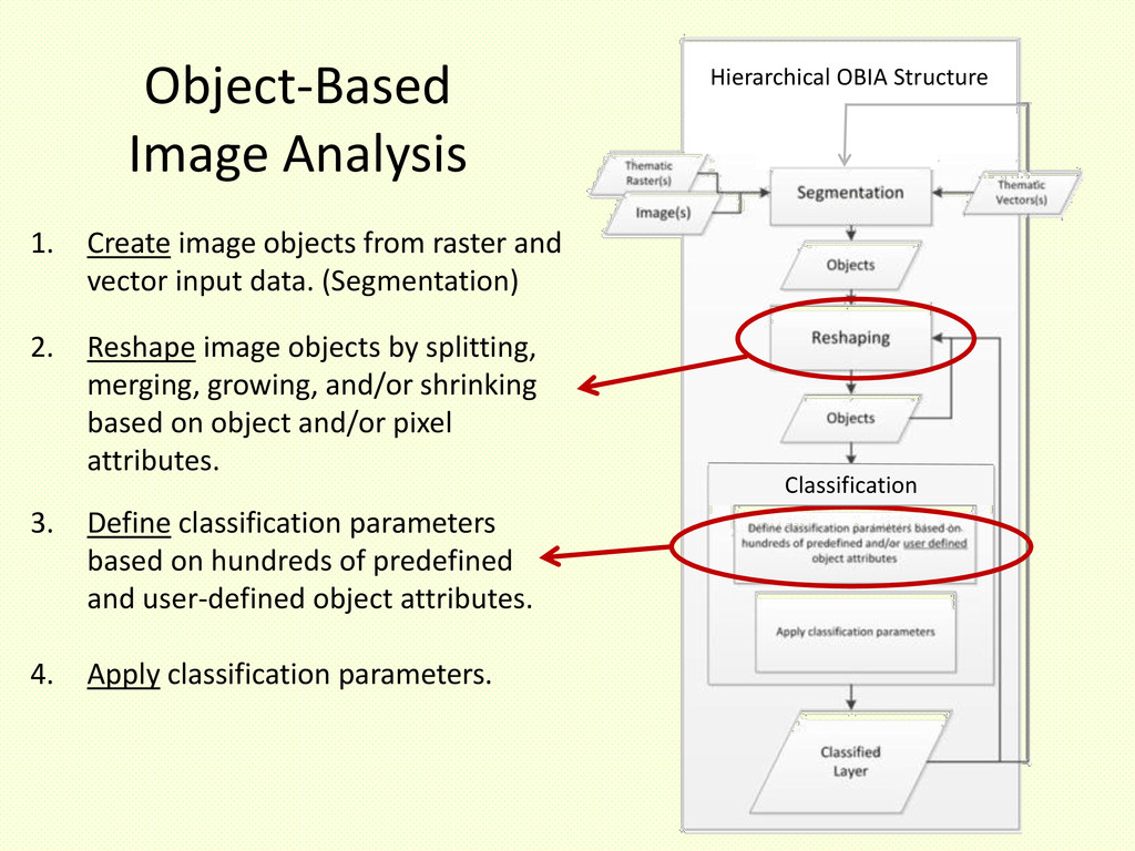
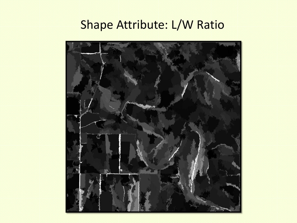
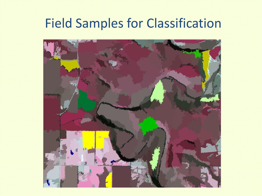
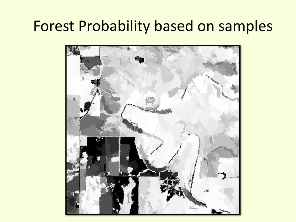
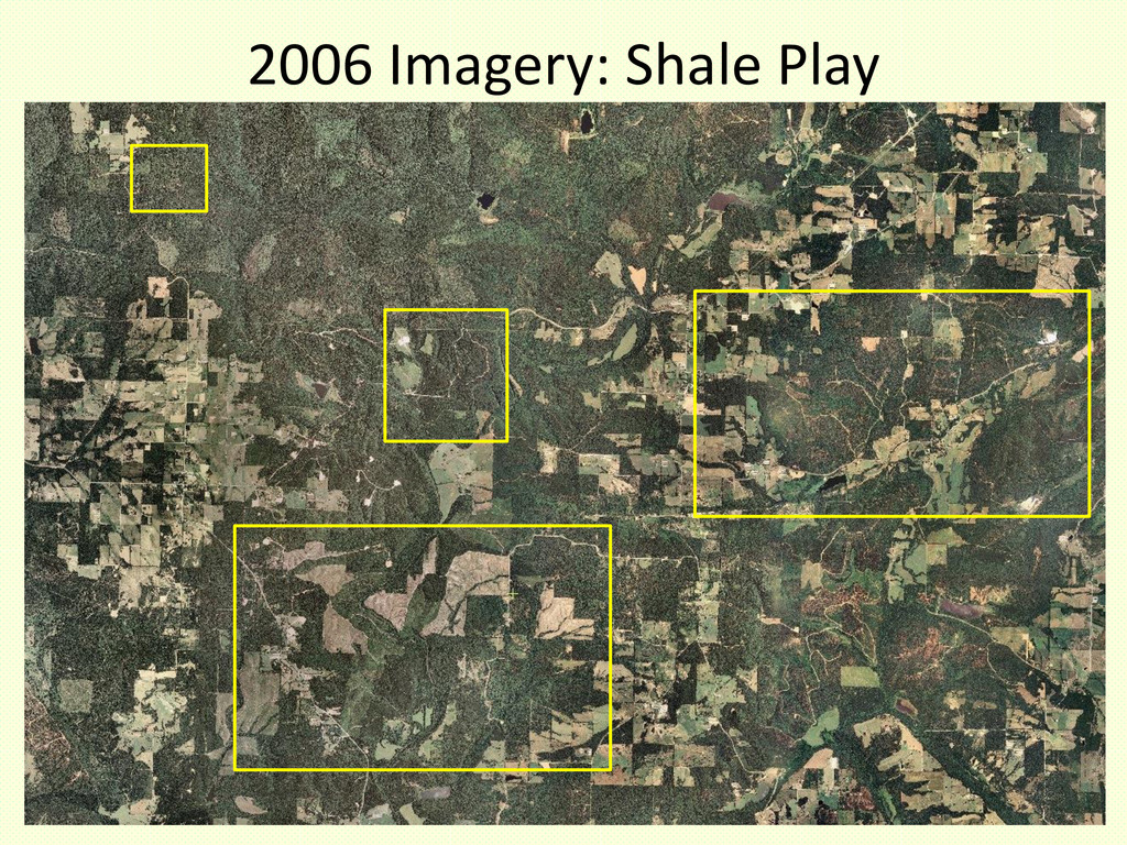
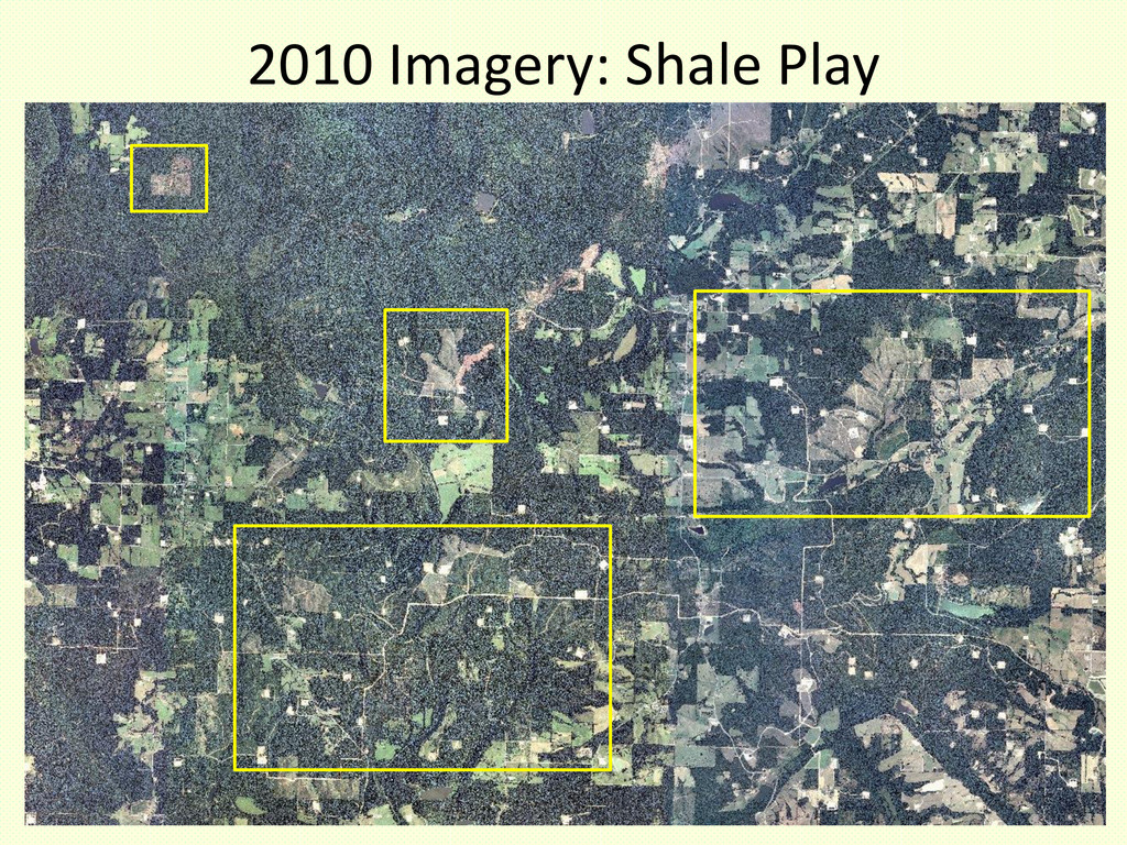
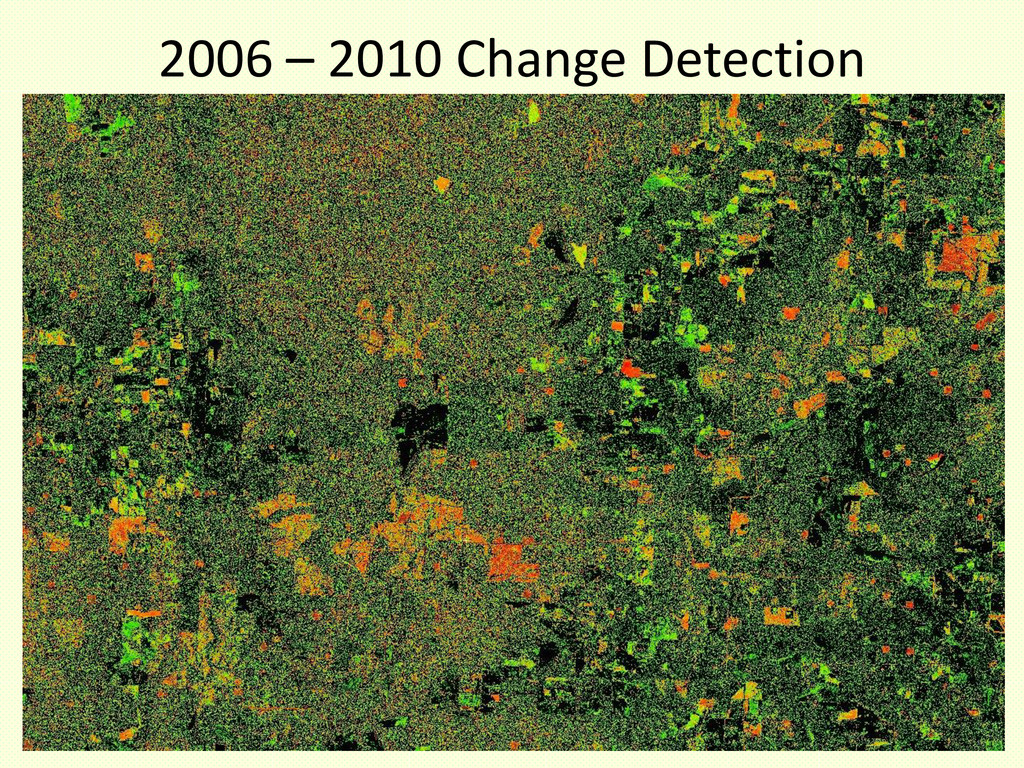
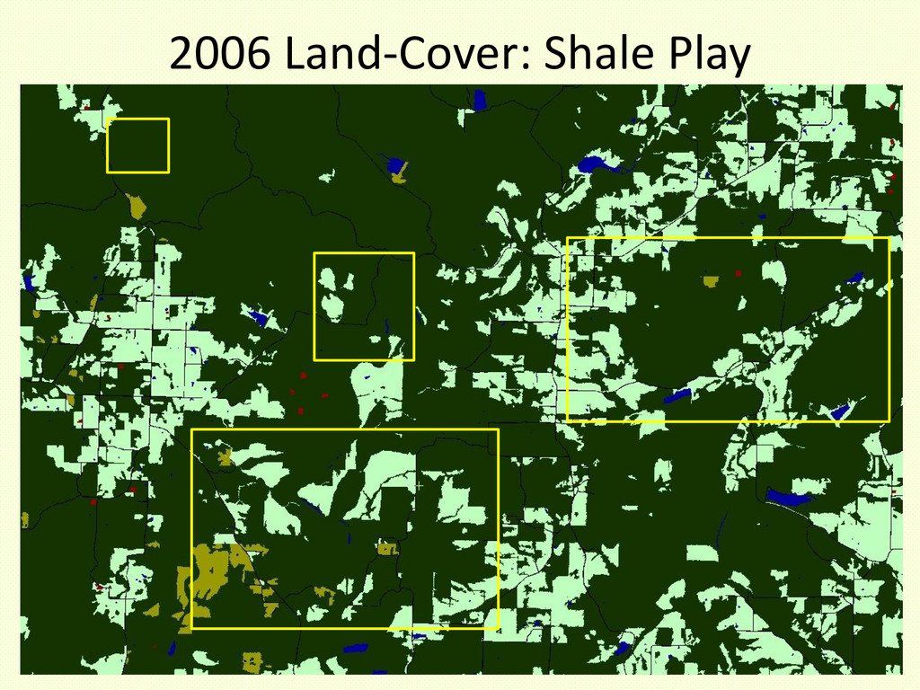
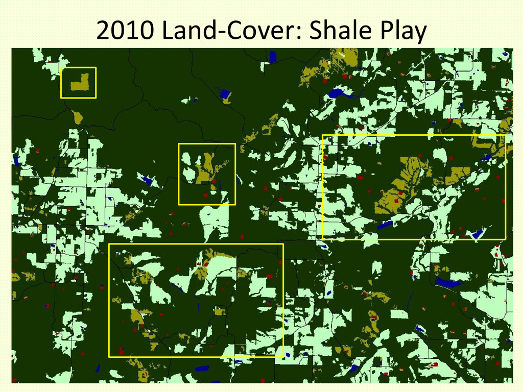
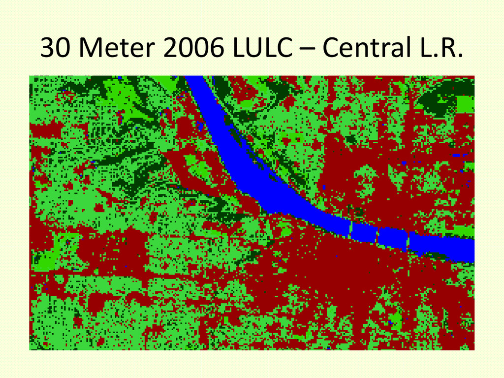
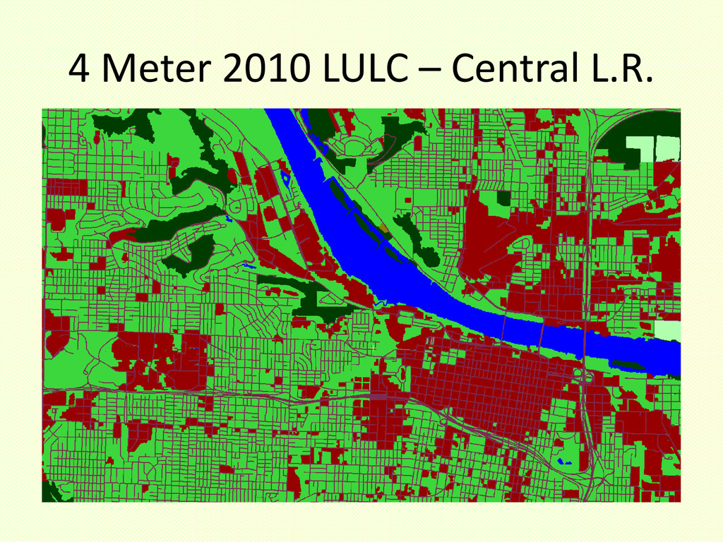
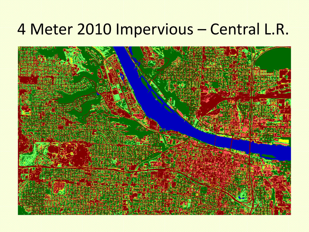
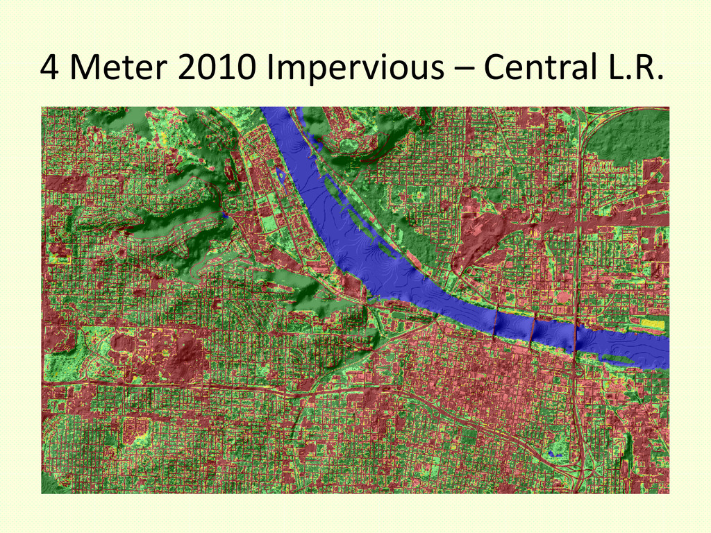
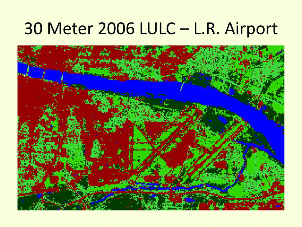
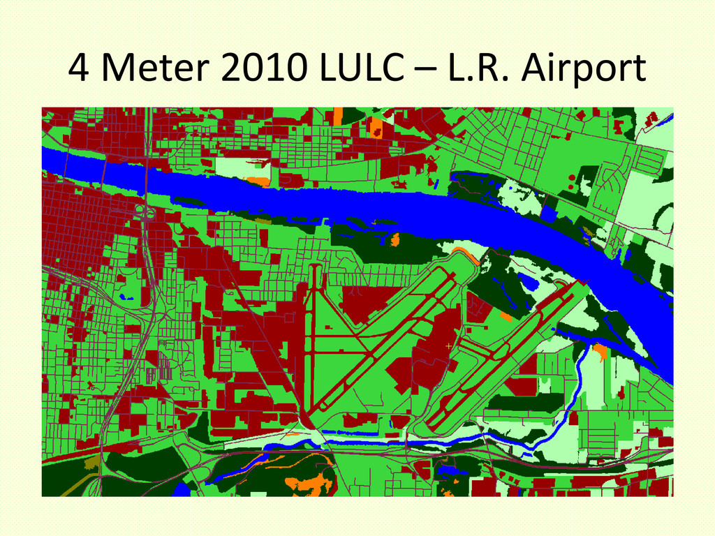
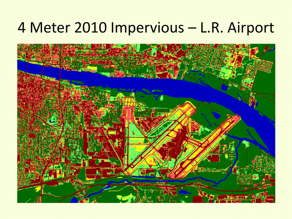
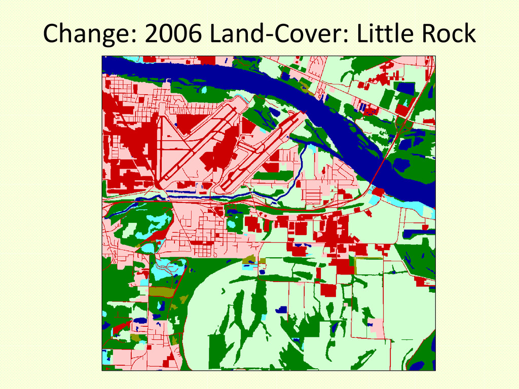
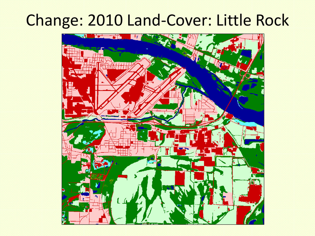
Digital photographic imagery from USDA’s NAIP (National Agriculture Imagery Program) is used extensively for various applications such as natural resource and environmental management, urban planning, etc. These applications are usually limited to small-scale, manual digitization procedures. NAIP imagery, however, provides interesting possibilities for use as primary input data for large-scale and automated land-cover mapping. Although NAIP 4-band imagery lacks the spectral resolution for efficiently extracting land-use information using pixel-based classification methods, geo-objectbased image analysis techniques (GEOBIA), which incorporate image characteristics such as texture, proximity, and shape, can be practical for land-cover mapping from aerial imagery. Between July 2009 and June 2013, the Arkansas Land-use/Land-cover (LULC) project developed automated processes for LULC classification from high-resolution images employing GEOBIA techniques. This presentation covers the automated extraction of land-cover information from two dates of NAIP imagery {2006 and 2010) as well as the methodologies developed for mapping land-cover changes between the two dates.

Transcript

1. Multi-Date Land-Cover Mapping with NAIP Imagery Arkansas 2006-2010 Arkansas GIS User Symposium 9:00 A.M., September 12, 2013
2. Project Funding and Cooperators • Arkansas General Improvement Fund • Ark. Natural Heritage Commission • ArkansasView & AmericaView • PCI Geomatics University Alliance • Trimble Navigation LTD. eCognition • University of Arkansas – CAST
3. A Little History 1990s • 1993 – 1995 Arkansas GAP Analysis Land-Cover – Based on 1992 Landsat Imagery – Focus primarily on Forest • 1997 – 1998 Mississippi Alluvial Valley LULC – Based on 3 Seasons of 1992 Landsat and MODIS Imagery – Detailed Agriculture Layer to Augment GAP • 1999 – 2002 Arkansas LULC 1999 – Based on 3 Seasons of 1999 Landsat Imagery – 3 Season Land-cover and Forest Updates
4. A Little History 2000s • 2005 – 2006 Arkansas LULC 2004 – Based on 3 Seasons of 2004 Landsat Imagery – 3 Season Land-cover and Forest Updates • 2006 – 2007 Arkansas LULC 2006 – Limited Update of LULC 2004 • 2008 – 2011 Small Area Land-Cover with Aerial Photography. (Work with ANHC) – Extensive Field Work – Very Small in Scale
5. Arkansas Land-Cover High Resolution Approach 2009 - Present • Source Imagery – Aerial Photography • 2006 Statewide High Resolution Land-Cover (Completed, Available via FTP) http://cast-ftp1.cast.uark.edu/bruce/ARKANSAS_HIRES/2006_LULC_QQs/ • 2010 Statewide High Resolution Land-Cover and Impervious Surface (Select Availability)
6. Mountain Home – 2006 4M Land-Cover
7. Aerial Photography Sources • ADOP 2006: Color-IR, 1 meter pixels, Winter • NAIP 2006: Real Color, 2 meter pixels, Summer • NAIP 2010: Color-IR, 1 meter pixels, Summer  NAIP = National Agriculture Imagery Program (USDA)  ADOP = Arkansas Digital Ortho Program (AGIO)
8. New Data Specifications • Spatial Resolution 4 Meters • 8 Land-Cover Categories • Organized by Quarter-Quad (based on USGS 7.5 minute quadrangle series) • Currently available in Raster format
9. High Resolution… ? • In our case 4 meter spatial resolution • Low by some standards where a high degree of spatial precision is needed: Cadastral Mapping, etc. • High in the field of Land-cover mapping. • Low at a scale for mapping facilities or cities. • Very High at a scale for mapping entire states.
10. Categorical Detail Roads Water Agriculture/Grass Forest/Woodland Urban Low Intensity Urban High Intensity Transitional Barren 2010 Northwestern Little Rock
11. Category Description Roads • Derived from Classified Imagery and Arkansas Centerlines • Paved and Unpaved Water • Derived from Classified Imagery Only • Includes Aquaculture Ponds (in Use), Lakes, and Large Streams Agriculture/Grass • Derived from Classified Imagery Only • Includes Pastures, Fields, Lawns, Cropland • May Also Include Large Urban Green Spaces: Parks, Cemeteries, etc. Forest/Woodland • Derived from Classified Imagery Only • This is Basically a Tree Canopy Map (Excepting Road Centerlines)
12. Category Description Urban Low Intensity • Derived from Classified Imagery and Parcel Polygons (Where Available) • Mix of Permeable and Impervious Surfaces • Includes Residential, Low Impact Commercial, etc. Urban High Intensity • Derived from Classified Imagery and Parcel Polygons (Where Available) • Impervious Surfaces of Various Kinds • Includes Commercial, Industrial, Parking Lots, Agricultural Processing, etc.
13. Category Description Transitional • Derived from Classified Imagery • Areas in Transition • Includes Forest Cuts, Pasture/Cropland Conversion, Urban Fringe Conversion, etc. Barren • Derived from Classified Imagery • Areas of Bare Earth • Includes Sandbars, Beaches, Construction, Gravel Pits, Mining, etc.
14. Study Area
15. Study Area
16. Study Area-Related Challenges • Size of Study Area: – Aerial Imagery made over an extended period of time. • Brightness and Contrast can significantly – Lots of Data! • Diversity of Landscape: – Arkansas has a very diverse landscape. – Individual Landscape Types are often Complex • OBIA Rules-Based Classification Demands: – Rules require us to know a lot about the landscape. – The more we know, the better our rules will be.
17. Topography and Morphology • Vegetation Type • Shadowing
18. Climate • Generally, Drier in North and West. Especially Northwest. • Generally, Wetter in South and East. • Anomalies
19. Seasonal Variability across Arkansas Fayetteville Crossett
20. Soils • Soils determine, to a great degree, where particular plants can and cannot grow.
21. Mapping the State by Ecoregion • There’s not a separate rule-set for each ecoregion. • Final output category, however, is weighted by overlap with a particular ecoregion. • Examples: • Bare Soil in Delta • Transitional in Pine Forests of GCP and Southern Boston Mts. vs. Cropland and Pasturelands.
22. Mapping Areas by Population Density and Urbanization Levels. • No separate rule-set for Urban Areas. • Final output category, however, is weighted by proximity to urban area and by information contained in parcel database (where available).
23. General Model Preparation Input Data to Model Imagery Streams Elevation Roads ∙ Slope ∙ Aspect ∙ Slope Position ∙ Stream Buffer ∙ Stream Order ∙ Image Segments Data Preprocessing OBIA Rule-Set Analysis Preliminary Output Maps Accuracy Assessment Final Output Maps Accuracy Data Training Data Collect and Process Field Data
24. Preparation • Assign Project Personnel • Define Each Category (Habitat) to be Mapped. • Identify and Acquire Needed Data Inputs` • Determine Data Processing Requirements and Configure System Preparation Input Data to Model Imagery Streams Elevation Roads ∙ Slope ∙ Aspect ∙ Slope Position ∙ Stream Buffer ∙ Roads Buffer ∙ Image Segments Data Preprocessing OBIA Rule-Set Analysis Preliminary Output Maps Accuracy Assessment Final Output Maps Accuracy Data Training Data Collect and Process Field Data
25. Field Work • Planning Phase: 1) Data Collection 2) Routes 3) Sampling Method 4) Hardware Check 5) Logistics • Data Collection Phase • Field Data Processing: Split Data Points into Two Data-Sets: 1) Training Data as Input to the Habitat Classification 2) Accuracy Assessment Data for Checking the Quality of the Output Maps. Preparation Input Data to Model Imagery Streams Elevation Roads ∙ Slope ∙ Aspect ∙ Slope Position ∙ Stream Buffer ∙ Roads Buffer ∙ Image Segments Data Preprocessing OBIA Rule-Set Analysis Preliminary Output Maps Accuracy Assessment Final Output Maps Accuracy Data Training Data Collect and Process Field Data
26. Field Data April 2007, March 2008, April 2009, March 2010, and July/August 2011 (With ANHC, Foti and Akin)
29. Two Uses for Ground Reference Data • Samples tell us about common characteristics that exist within and between categories. • Similar Reflectance Values • Similar Topography • Relationships to Streams and Roads • Similar Geographic Distribution • To determine the final accuracy of the maps. After the maps have been completed we can compare our ground samples to the computer-produced map. From this we can: • Determine the accuracy of the map • Determine the accuracy of individual categories in the map • Improve future modeling processes as a whole
30. Data Input • Import Datasets • Geo-Reference (Co- Register) Datasets • Data Quality Assurance and Control • Proper Formatting • Set Computer Network Linkages Preparation Input Data to Model Imagery Streams Elevation Roads ∙ Slope ∙ Aspect ∙ Slope Position ∙ Stream Buffer ∙ Roads Buffer ∙ Image Segments Data Preprocessing OBIA Rule-Set Analysis Preliminary Output Maps Accuracy Assessment Final Output Maps Accuracy Data Training Data Collect and Process Field Data
31. Image Rectification and/or Transformation The process of make two or more images register by transforming image data pixels from one grid system into another using a standard set of geographic coordinates and re-sampling algorithms, or by transforming the projection/datum between raster and vector spatial datasets. Image 1 Image 2 Image 1 Rectified to register with Image 2
32. Registered (Georeferenced) Data
33. Data Preprocessing • Create Needed Datasets from Input Imagery Preparation Input Data to Model Imagery Streams Elevation Roads Slope Aspect Stream Buffer Road Buffer Initial Image Segments Data Preprocessing OBIA Rule-Set Analysis Preliminary Output Maps Accuracy Assessment Final Output Maps Accuracy Data Training Data Collect and Process Field Data
34. Topography ASPECT SLOPE
35. Buffering Streams Roads
36. Initial Segmentation: Object Polygons
37. OBIA Analysis • Develop Rulesets based on input data thresholds. • Design and Implement Grid Network. • Assign Categories to Object Polygons (Segments). • Filter and “Clean-Up” Output Maps. Preparation Input Data to Model Imagery Streams Elevation Roads ∙ Slope ∙ Aspect ∙ Slope Position ∙ Stream Buffer ∙ Stream Order ∙ Image Segments Data Preprocessing OBIA Rule-Set Analysis Preliminary Output Maps Accuracy Assessment Final Output Maps Accuracy Data Training Data Collect and Process Field Data
38. Object-Based Image Analysis 3. Define classification parameters based on hundreds of predefined and user-defined object attributes. 4. Apply classification parameters. 1. Create image objects from raster and vector input data. (Segmentation) 2. Reshape image objects by splitting, merging, growing, and/or shrinking based on object and/or pixel attributes. Hierarchical OBIA Structure Classification
39. Initial Segmentation: Object Polygons
40. Subsequent Segmentation: Smaller Object Polygons
41. These Objects Have Attributes • Out of the Box • Customized
42. Texture Attribute: Contrast
43. Shape Attribute: L/W Ratio
44. Field Samples for Classification
45. Forest Probability based on samples
46. Grid Computing • Once all data is in place and pre-processed. • Hi-Resolution Images at Statewide Scale requires large data handling capability. • Multiple Computer Nodes (Cores) in a Networked Grid Job Scheduler
47. Segments Classified By Attributes Low
48. Data Preprocessing • Assess Accuracy or Preliminary Maps by Comparing Ground Reference Samples to Classified Maps. • Calculate Accuracy Statistics Preparation Input Data to Model Imagery Streams Elevation Roads ∙ Slope ∙ Aspect ∙ Slope Position ∙ Stream Buffer ∙ Stream Order ∙ Image Segments Data Preprocessing OBIA Rule-Set Analysis Preliminary Output Maps Accuracy Assessment Final Output Maps Accuracy Data Training Data Collect and Process Field Data
49. Accuracy from Ground Reference • Limited Ground Reference Coverage Needs more work in: •Mississippi Alluvial Valley •Gulf Coastal Plain •Needs more GR points everywhere • Plans for Community Sourcing (We could use the help).
50. Where We Stand Now • 2006 – 4-Meter Statewide LULC Available http://cast-ftp1.cast.uark.edu/bruce/ARKANSAS_HIRES/2006_LULC_QQs/ • 2010 – 4 Meter LULC Partial Availability – Contact Me for Availability & Updates – Standardization and Final Formatting
51. 2006 Imagery: Shale Play
52. 2010 Imagery: Shale Play
53. 2006 – 2010 Change Detection
54. 2006 Land-Cover: Shale Play
55. 2010 Land-Cover: Shale Play
56. 30 Meter 2006 LULC – Central L.R.
57. 4 Meter 2010 LULC – Central L.R.
58. 4 Meter 2010 Impervious – Central L.R.
59. 4 Meter 2010 Impervious – Central L.R.
60. 30 Meter 2006 LULC – L.R. Airport
61. 4 Meter 2010 LULC – L.R. Airport
62. 4 Meter 2010 Impervious – L.R. Airport
63. 4 Meter 2010 Impervious – L.R. Airport
64. Change: 2006 Land-Cover: Little Rock
65. Change: 2010 Land-Cover: Little Rock
66. Future Directions • Change Detection Maps (In the Works) • Web Services (In the Works) • Ground Reference Network • 2013 NAIP Updates? • Higher Resolution in Metro Areas? • Greater Categorical Detail…
67. Greater Categorical Detail Water Deciduous Cool Season Grasses Urban/Built-up Evergreen Barren Warm Season Grasses Transitional Crops Breakout ??? Other Categories???