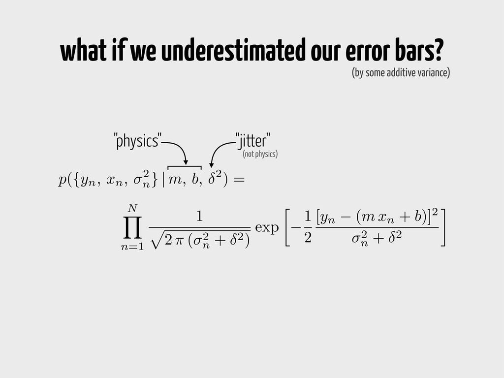
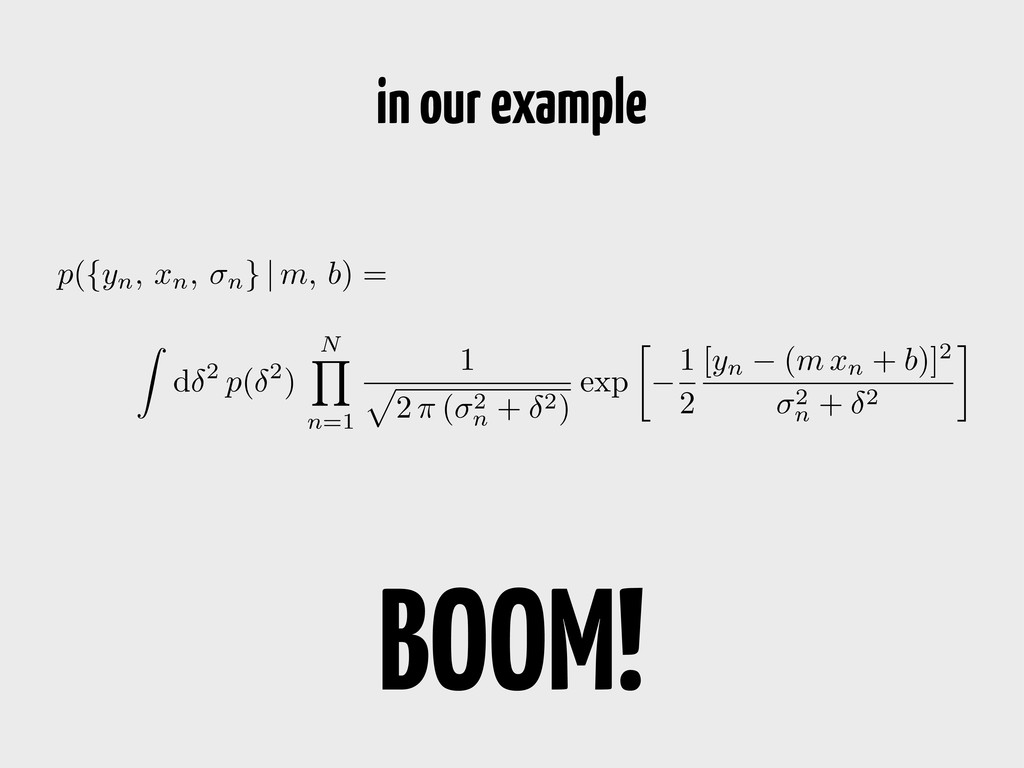
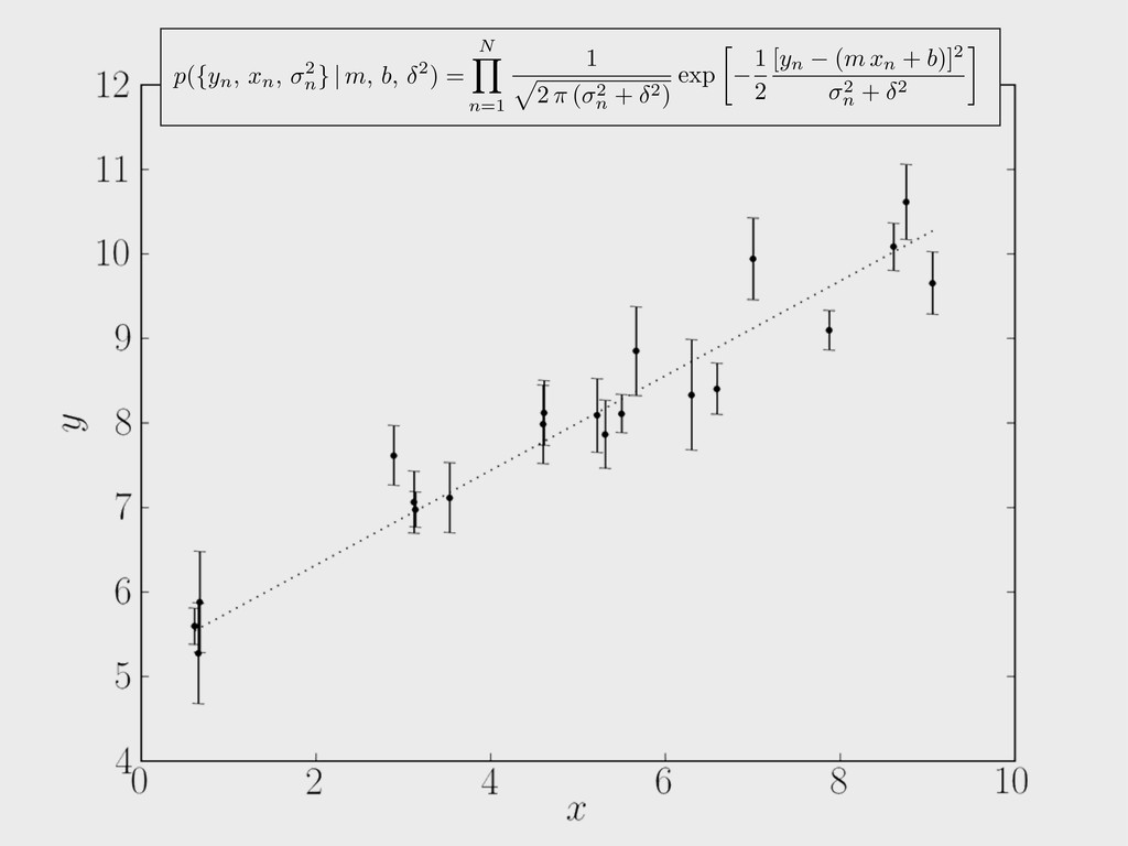
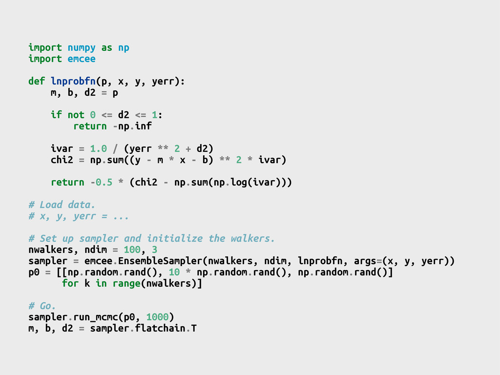
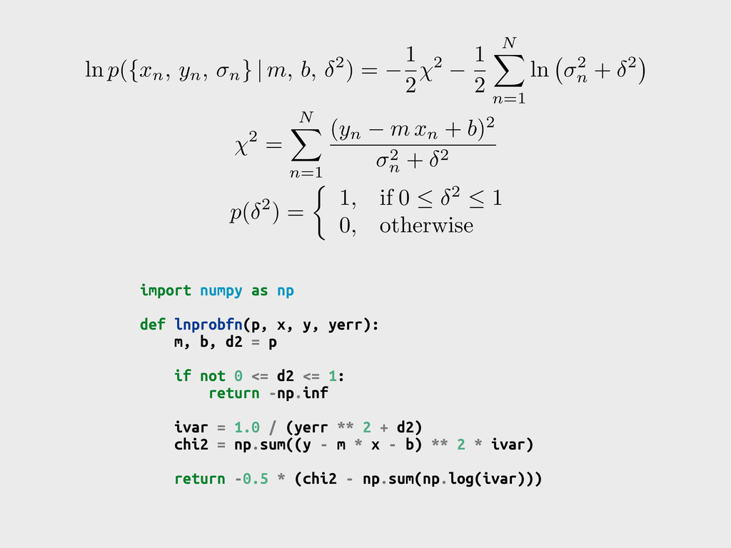
b, d2 = p if not 0 <= d2 <= 1: return -np.inf ivar = 1.0 / (yerr ** 2 + d2) chi2 = np.sum((y - m * x - b) ** 2 * ivar) return -0.5 * (chi2 - np.sum(np.log(ivar))) p ( 2 ) = ⇢ 1 , if 0 2 1 0 , otherwise 2 = N X n=1 ( yn m xn + b )2 2 n + 2 ln p ({ xn, yn, n } | m, b, 2) = 1 2 2 1 2 N X n=1 ln 2 n + 2
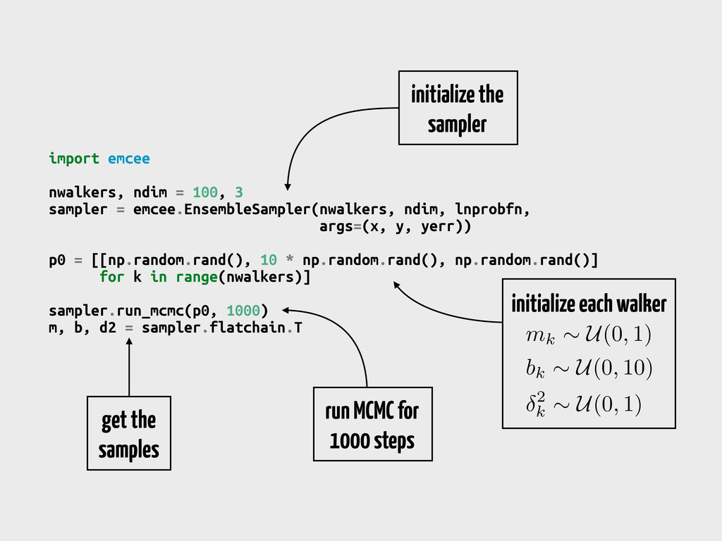
ndim, lnprobfn, args=(x, y, yerr)) p0 = [[np.random.rand(), 10 * np.random.rand(), np.random.rand()] for k in range(nwalkers)] sampler.run_mcmc(p0, 1000) m, b, d2 = sampler.flatchain.T mk ⇠ U(0, 1) bk ⇠ U(0, 10) 2 k ⇠ U(0, 1) initialize each walker run MCMC for 1000 steps get the samples initialize the sampler
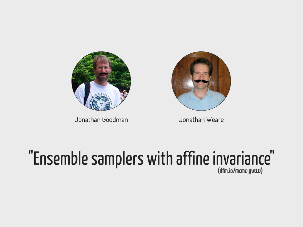
Meierjurgen Farr (Northwestern) David W. Hogg (NYU) Dustin Lang (CMU) Phil Marshall (Oxford) Ilya Pashchenko (ASC LPI, Moscow) Adrian Price-Whelan (Columbia) Jeremy Sanders (Cambridge) Joe Zuntz (Oxford) Eric Agol (UW) Jo Bovy (IAS) Jacqueline Chen (MIT) John Gizis (Delaware) Jonathan Goodman (NYU) Marius Millea (UC Davis) Jennifer Piscionere (Vanderbilt) contributors
Meierjurgen Farr (Northwestern) David W. Hogg (NYU) Dustin Lang (CMU) Phil Marshall (Oxford) Ilya Pashchenko (ASC LPI, Moscow) Adrian Price-Whelan (Columbia) Jeremy Sanders (Cambridge) Joe Zuntz (Oxford) Eric Agol (UW) Jo Bovy (IAS) Jacqueline Chen (MIT) John Gizis (Delaware) Jonathan Goodman (NYU) Marius Millea (UC Davis) Jennifer Piscionere (Vanderbilt) thanks!
![What do you really want? Ep[f(✓)] = 1 Z Z](https://files.speakerdeck.com/presentations/1cbbeda07de1013062221231381d8c65/slide_20.jpg)
![probably. What do you really want? Ep[f(✓)] = 1 Z](https://files.speakerdeck.com/presentations/1cbbeda07de1013062221231381d8c65/slide_21.jpg)
![Ep[f(✓)] = 1 Z Z f(✓) p(✓) p(D | ✓)](https://files.speakerdeck.com/presentations/1cbbeda07de1013062221231381d8c65/slide_22.jpg)
![Ep[f(✓)] = 1 Z Z f(✓) p(✓) p(D | ✓)](https://files.speakerdeck.com/presentations/1cbbeda07de1013062221231381d8c65/slide_23.jpg)
![Ep[f(✓)] = 1 Z Z f(✓) p(✓) p(D | ✓)](https://files.speakerdeck.com/presentations/1cbbeda07de1013062221231381d8c65/slide_24.jpg)
![Ep[f(✓)] = 1 Z Z f(✓) p(✓) p(D | ✓)](https://files.speakerdeck.com/presentations/1cbbeda07de1013062221231381d8c65/slide_25.jpg)
![emcee has a live support team. [email protected]](https://files.speakerdeck.com/presentations/1cbbeda07de1013062221231381d8c65/slide_121.jpg)