Upgrade to Pro — share decks privately, control downloads, hide ads and more …

SAMSI QMC Transition 2018 May

SAMSI QMC Transition 2018 May

SAMSI QMC Transition Workshop Talk on approximating functions whose values are expensive

Fred J. Hickernell

May 07, 2018
Tweet

More Decks by Fred J. Hickernell

Other Decks in Research

Transcript

  1. Function Approximation When Function Values Are Expensive Fred J. Hickernell1

    Simon Mak2 1Department of Applied Mathematics, Illinois Institute of Technology, [email protected] 2School of Industrial and System Engineering, Georgia Institute of Technology Supported by NSF-DMS-1522687 and DMS-1638521 (SAMSI) SAMSI-QMC Transition Workshop, May 7, 2018
  2. Background Approx. by Series Coefficients Approx. by Function Values References

    Appendix Thanks to ... SAMSI for sponsoring this program in Quasi-Monte Carlo Methods and High Dimensional Sampling for Applied Mathematics Especially Ilse Ipsen, Karem Jackson, Sue McDonald, Rick Scoggins, Thomas Gehrmann, Richard Smith, and David Banks 2/25
  3. Background Approx. by Series Coefficients Approx. by Function Values References

    Appendix Thanks to ... SAMSI for sponsoring this program in Quasi-Monte Carlo Methods and High Dimensional Sampling for Applied Mathematics Especially Ilse Ipsen, Karem Jackson, Sue McDonald, Rick Scoggins, Thomas Gehrmann, Richard Smith, and David Banks Frances Kuo, Pierre L’Ecuyer, and Art Owen, fellow program leaders Especially Art, who keeps trying to push QMC out of its box 2/25
  4. Background Approx. by Series Coefficients Approx. by Function Values References

    Appendix Thanks to ... SAMSI for sponsoring this program in Quasi-Monte Carlo Methods and High Dimensional Sampling for Applied Mathematics Especially Ilse Ipsen, Karem Jackson, Sue McDonald, Rick Scoggins, Thomas Gehrmann, Richard Smith, and David Banks Frances Kuo, Pierre L’Ecuyer, and Art Owen, fellow program leaders Especially Art, who keeps trying to push QMC out of its box Many of you with whom I have had fruiful discussions, especially WGs 2, 4, and 5 2/25
  5. Background Approx. by Series Coefficients Approx. by Function Values References

    Appendix Thanks to ... SAMSI for sponsoring this program in Quasi-Monte Carlo Methods and High Dimensional Sampling for Applied Mathematics Especially Ilse Ipsen, Karem Jackson, Sue McDonald, Rick Scoggins, Thomas Gehrmann, Richard Smith, and David Banks Frances Kuo, Pierre L’Ecuyer, and Art Owen, fellow program leaders Especially Art, who keeps trying to push QMC out of its box Many of you with whom I have had fruiful discussions, especially WGs 2, 4, and 5 Mac Hyman, who Promoted QMC to SAMSI behind the scenes Introduced me to problems with expensive function values Co-led WG 5 2/25
  6. Background Approx. by Series Coefficients Approx. by Function Values References

    Appendix Thanks to ... SAMSI for sponsoring this program in Quasi-Monte Carlo Methods and High Dimensional Sampling for Applied Mathematics Especially Ilse Ipsen, Karem Jackson, Sue McDonald, Rick Scoggins, Thomas Gehrmann, Richard Smith, and David Banks Frances Kuo, Pierre L’Ecuyer, and Art Owen, fellow program leaders Especially Art, who keeps trying to push QMC out of its box Many of you with whom I have had fruiful discussions, especially WGs 2, 4, and 5 Mac Hyman, who Promoted QMC to SAMSI behind the scenes Introduced me to problems with expensive function values Co-led WG 5 Henryk Woźniakowski, whose work on tractability has inspired some of what I will say 2/25
  7. Background Approx. by Series Coefficients Approx. by Function Values References

    Appendix Thanks to ... SAMSI for sponsoring this program in Quasi-Monte Carlo Methods and High Dimensional Sampling for Applied Mathematics Especially Ilse Ipsen, Karem Jackson, Sue McDonald, Rick Scoggins, Thomas Gehrmann, Richard Smith, and David Banks Frances Kuo, Pierre L’Ecuyer, and Art Owen, fellow program leaders Especially Art, who keeps trying to push QMC out of its box Many of you with whom I have had fruiful discussions, especially WGs 2, 4, and 5 Mac Hyman, who Promoted QMC to SAMSI behind the scenes Introduced me to problems with expensive function values Co-led WG 5 Henryk Woźniakowski, whose work on tractability has inspired some of what I will say Kai-Tai Fang, who introduced me to experimental design 2/25
  8. Background Approx. by Series Coefficients Approx. by Function Values References

    Appendix Approximating Functions When Function Values Are Expensive Interested in f : [−1, 1]d → R, e.g., the result of a climate model, or a financial calculation d is dozens or a few hundred $(f) = cost to evaluate f(x) for any x ∈ [−1, 1]d = hours or days or $1M Want to construct a surrogate model, fapp ≈ f, with $(fapp) = $0.000001 so that we may quickly explore (plot, integrate, optimize, search for sharp gradients of) f fapp is constructed using n pieces of information about f Want f − fapp ∞ ε for n = O(dpε−q) as d ↑ ∞ or ε ↓ 0 (with small p and q) Assume $(f) nr for any practical n and any positive r, so the cost of the algorithm is O($(f)n) 3/25
  9. Background Approx. by Series Coefficients Approx. by Function Values References

    Appendix Functions Expressed at Series Let f : [−1, 1]d → R have L2([−1, 1]d, ) an orthogonal series expansion: f(x) = j∈Nd 0 f(j)φj(x), φj(x) = φj1 (x1) · · · φjd (xd), φj ∞ = 1 f(j) = f, φj φj, φj , f, g := [−1,1]d f(x)g(x) (x) dx Legendre polynomials: 1 −1 φj(x)φk(x) dx = cjδj,k Chebyshev polynomials: φj(x) = cos(j arccos(x)), 1 −1 φj(x)φk(x) √ 1 − x2 dx = cjδj,k 4/25
  10. Background Approx. by Series Coefficients Approx. by Function Values References

    Appendix Approximation by Series Coefficients f(x) = j∈Nd 0 f(j)φj(x), f(j) = f, φj φj, φj , φj ∞ = 1 Suppose that we may observe the series coefficients f(j) at a cost of $1M each. (Eventually we want to consider the case of observing function values.) For any vector of non-negative constants, γ = (γj)j∈Nd 0 , define the norm f q,γ := f(j) γj j∈Nd 0 q , 0/0 = 0, γj = 0 & f ∞,γ < ∞ =⇒ f(j) = 0 Order the wavenumbers j such that γj1 γj2 · · · . The optimal approximation why? to f given the choice of n series coefficients is fapp(x) = n i=1 f(ji)φji , f − fapp ∞ = ∞ i=n+1 f(ji)φji ∞ loose f−fapp 1 tight optimal f ∞,γ ∞ i=n+1 γji 6/25
  11. Background Approx. by Series Coefficients Approx. by Function Values References

    Appendix How Quickly Does Error Decay? f(x) = j∈Nd 0 f(j)φj(x), f(j) = f, φj φj, φj , φj ∞ = 1, f q,γ = f(j) γj j∈Nd 0 q γj1 γj2 · · · , fapp(x) = n i=1 f(ji)φji , f − fapp ∞ loose f − fapp 1 tight optimal f ∞,γ ∞ i=n+1 γji An often used trick (q > 0): γjn+1 1 n γ1/q j1 + · · · + γ1/q jn q 1 nq γ 1/q , γ 1/q = j∈Nd 0 γ1/q j q ∞ i=n+1 γji γ 1/q ∞ i=n 1 iq γ 1/q (q − 1)(n − 1)q−1 rate controlled by finiteness of γ 1/q 7/25
  12. Background Approx. by Series Coefficients Approx. by Function Values References

    Appendix Recap f(x) = j∈Nd 0 f(j)φj(x), f(j) = f, φj φj, φj , φj ∞ = 1, f q,γ = f(j) γj j∈Nd 0 q dependence of f on d is hidden γj1 γj2 · · · , fapp(x) = n i=1 f(ji)φji , f − fapp ∞ f − fapp 1 f ∞,γ ∞ i=n+1 γji f ∞,γ γ 1/q (q − 1)(n − 1)q−1 Want ε n = O      f ∞,γ γ 1/q ε   1/(q−1)   is sufficient To succeed with n = O(dp) , we need γ 1/q = O(dp ) Novak, E. & Woźniakowski, H. Tractability of Multivariate Problems Volume I: Linear Information. EMS Tracts in Mathematics 6 (European Mathematical Society, Zürich, 2008), Kühn, T. et al. Approximation numbers of Sobolev embeddings—Sharp constants and tractability. J. Complexity 30, 95–116 (2014). 8/25
  13. Background Approx. by Series Coefficients Approx. by Function Values References

    Appendix Recap f(x) = j∈Nd 0 f(j)φj(x), f(j) = f, φj φj, φj , φj ∞ = 1, f q,γ = f(j) γj j∈Nd 0 q dependence of f on d is hidden γj1 γj2 · · · , fapp(x) = n i=1 f(ji)φji , f − fapp ∞ f − fapp 1 f ∞,γ ∞ i=n+1 γji f ∞,γ γ 1/q (q − 1)(n − 1)q−1 Want ε γ 1/q = O(dp ) =⇒ n = O(dp) What remains? 8/25
  14. Background Approx. by Series Coefficients Approx. by Function Values References

    Appendix Recap f(x) = j∈Nd 0 f(j)φj(x), f(j) = f, φj φj, φj , φj ∞ = 1, f q,γ = f(j) γj j∈Nd 0 q dependence of f on d is hidden γj1 γj2 · · · , fapp(x) = n i=1 f(ji)φji , f − fapp ∞ f − fapp 1 f ∞,γ ∞ i=n+1 γji f ∞,γ γ 1/q (q − 1)(n − 1)q−1 Want ε γ 1/q = O(dp ) =⇒ n = O(dp) What remains? How do we infer γ in practice? Tradition fixes something convenient. 8/25
  15. Background Approx. by Series Coefficients Approx. by Function Values References

    Appendix Recap f(x) = j∈Nd 0 f(j)φj(x), f(j) = f, φj φj, φj , φj ∞ = 1, f q,γ = f(j) γj j∈Nd 0 q dependence of f on d is hidden γj1 γj2 · · · , fapp(x) = n i=1 f(ji)φji , f − fapp ∞ f − fapp 1 f ∞,γ ∞ i=n+1 γji f ∞,γ γ 1/q (q − 1)(n − 1)q−1 Want ε γ 1/q = O(dp ) =⇒ n = O(dp) What remains? How do we infer γ in practice? Tradition fixes something convenient. How do we infer a bound on f ∞,γ ? 8/25
  16. Background Approx. by Series Coefficients Approx. by Function Values References

    Appendix Recap f(x) = j∈Nd 0 f(j)φj(x), f(j) = f, φj φj, φj , φj ∞ = 1, f q,γ = f(j) γj j∈Nd 0 q dependence of f on d is hidden γj1 γj2 · · · , fapp(x) = n i=1 f(ji)φji , f − fapp ∞ f − fapp 1 f ∞,γ ∞ i=n+1 γji f ∞,γ γ 1/q (q − 1)(n − 1)q−1 Want ε γ 1/q = O(dp ) =⇒ n = O(dp) What remains? How do we infer γ in practice? Tradition fixes something convenient. How do we infer a bound on f ∞,γ ? How do we approximate using function values, not series coefficients? 8/25
  17. Background Approx. by Series Coefficients Approx. by Function Values References

    Appendix Recap f(x) = j∈Nd 0 f(j)φj(x), f(j) = f, φj φj, φj , φj ∞ = 1, f q,γ = f(j) γj j∈Nd 0 q dependence of f on d is hidden γj1 γj2 · · · , fapp(x) = n i=1 f(ji)φji , f − fapp ∞ f − fapp 1 f ∞,γ ∞ i=n+1 γji f ∞,γ γ 1/q (q − 1)(n − 1)q−1 Want ε γ 1/q = O(dp ) =⇒ n = O(dp) What remains? Assume that the function is nice enough to allow this inference. How do we infer γ in practice? Tradition fixes something convenient. How do we infer a bound on f ∞,γ ? How do we approximate using function values, not series coefficients? 8/25
  18. Background Approx. by Series Coefficients Approx. by Function Values References

    Appendix Main New Ideas It is assumed that the f is nice enough to justify the following: Inferring γ Assume a structure informed by experimental design principles. Infer coordinate importance from a pilot sample with wavenumbers J := {(0, . . . , 0, j, 0 . . . , 0) : j = 0, . . . , n0} = {jek : j = 0, . . . , n0, k = 1, . . . , d} Inferring f ∞,γ Iteratively add wavenumber with largest γj to J. Inflate the norm that is observed so far and assume f ∞,γ C fj j∈J ∞,γ Function values Let the new wavenumber, j, pick the next design point via a shifted van der Corput sequence. Use interpolation to estimate fj j∈J . 9/25
  19. Background Approx. by Series Coefficients Approx. by Function Values References

    Appendix Product, Order, and Smoothness Dependent (POSD) Weights f(x) = j∈Nd 0 f(j)φj(x), f(j) = f, φj φj, φj , φj ∞ = 1, f q,γ = f(j) /γj j∈Nd 0 q j∈Nd 0 γ1/q j = O(dp ) =⇒ f − fapp ∞ ε for n = O(dp) if f ∞,γ < ∞ Experimental design assumes Effect sparsity: Only a small number of effects are important Effect hierarchy: Lower-order effects are more important than higher-order effects Effect heredity: Interaction is active only if both parent effects are also active Effect smoothness: Coarse horizontal scales are more important than fine horizontal scales Consider product, order, and smoothness dependent (POSD) weights: γj = Γ j 0 d =1 j >0 w sj , Γ0 = s1 = 1,      w = coordinate importance Γr = order size sj = smoothness degree Wu, C. F. J. & Hamada, M. Experiments: Planning, Analysis, and Parameter Design Optimization. (John Wiley & Sons, Inc., New York, 2000). 10/25
  20. Background Approx. by Series Coefficients Approx. by Function Values References

    Appendix Product, Order, and Smoothness Dependent Weights Effect sparsity: Only a small number of effects are important Effect hierarchy: Lower-order effects are more important than higher-order effects Effect heredity: Interaction is active only if both parent effects are also active Effect smoothness: Coarse horizontal scales are more important than fine horizontal scales Consider product, order and smoothness dependent weights: γj = Γ j 0 d =1 j >0 w sj , Γ0 = s1 = 1,      w = coordinate importance Γr = order size sj = smoothness degree j∈Nd 0 γ1/q j = u⊆1:d    Γ1/q |u| ∈u w1/q   ∞ j=1 s1/q j   |u|   = O(dp ) =⇒ f − fapp ∞ ε for n = O(dp) if f ∞,γ < ∞ 11/25
  21. Background Approx. by Series Coefficients Approx. by Function Values References

    Appendix Special Cases of Weights j∈Nd 0 γ1/q j = u⊆1:d    Γ1/q |u| ∈u w1/q   ∞ j=1 s1/q j   |u|   Want = O(dp ) Coordinates, orders equally important Γr = w = 1 j∈Nd 0 γ1/q j =  1 + ∞ j=1 s1/q j   d Fail Coordinates equally important No interactions w = Γ1 = 1, Γr = 0 ∀r > 1 j∈Nd 0 γ1/q j = 1 + d ∞ j=1 s1/q j Success Coordinates differ in importance Interactions equally important Γr = 1 j∈Nd 0 γ1/q j exp   ∞ k=1 w1/q k ∞ j=1 s1/q j   Success 12/25
  22. Background Approx. by Series Coefficients Approx. by Function Values References

    Appendix Algorithm When Both γ and f ∞,γ Are Inferred Require: Γ = vector of order sizes s = vector of smoothness degrees w∗ = max k wk n0 = minimum number of wavenumbers in each coordinate C = inflation factor f = a black-box series coefficient generator for the function of interest, f, where f ∞,γ C fj j∈J ∞,γ , J := {(0, . . . , 0, j, 0 . . . , 0) : j = 0, . . . , n0 } for all γ ε = positive absolute error tolerance Ensure: f − fapp ∞ ε 1: Evaluate f(j) for j ∈ J 2: Define w = min argmin w w∗ fj j∈J ∞,γ 3: Let n = min n : ∞ i=n +1 γji ε C fj j∈J ∞,γ 4: Compute fapp = n i=1 f(ji )φji Computational cost is n = O ε−1C f ∞,γ γ 1/q 1/(q−1) 14/25
  23. Background Approx. by Series Coefficients Approx. by Function Values References

    Appendix Example f manufactured in terms of random series coefficients 15/25
  24. Background Approx. by Series Coefficients Approx. by Function Values References

    Appendix A Gap Between Theory and Practice Theory using series coefficients Photo Credit: Xinhua Practice using function values 16/25
  25. Background Approx. by Series Coefficients Approx. by Function Values References

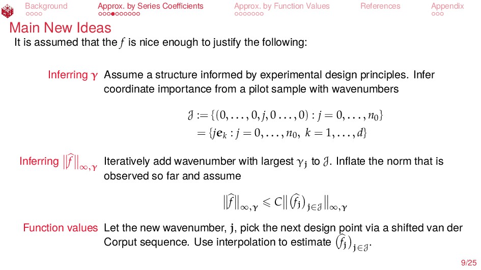
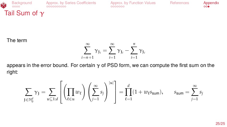
    Appendix A Very Sparse Grid on [−1, 1]d j 0 1 2 3 4 · · · van der Corput tj 0 1/2 1/4 3/4 1/8 · · · ψ(tj) := 2(tj + 1/3 mod 1) − 1 −1/3 2/3 1/6 −5/6 −1/12 · · · ψ(tj) := − cos(π(tj + 1/3 mod 1)) −0.5 0.8660 0.2588 −0.9659 −0.1305 · · · To estimate f(j), j ∈ J, use the design {(ψ(tj1 ), . . . , ψ(tjd ) : j ∈ J}. E.g., for J = {(0, 0, 0, 0), (1, 0, 0, 0), (0, 1, 0, 0), (0, 0, 1, 0), (0, 0, 0, 1), (2, 0, 0, 0), (3, 0, 0, 0), (1, 1, 0, 0)} Even Points ArcCos Points · · 17/25
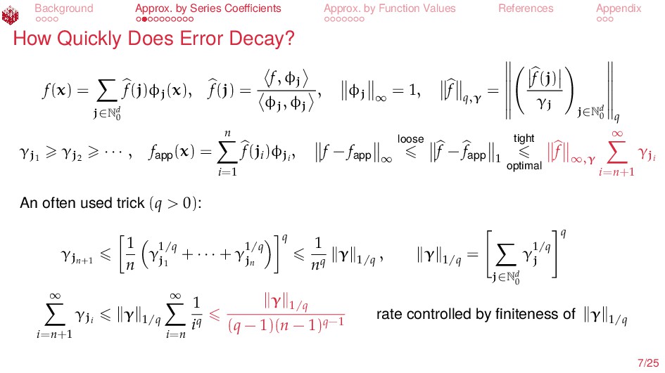
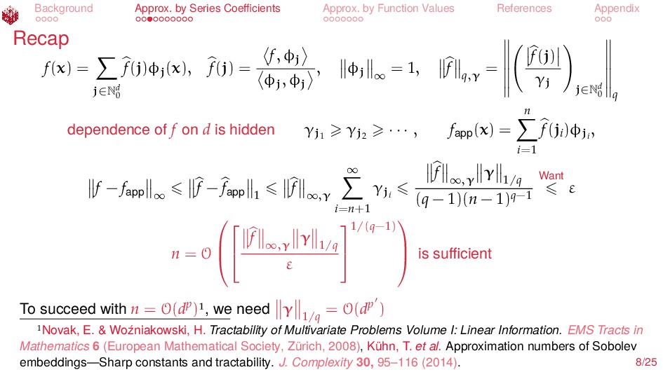
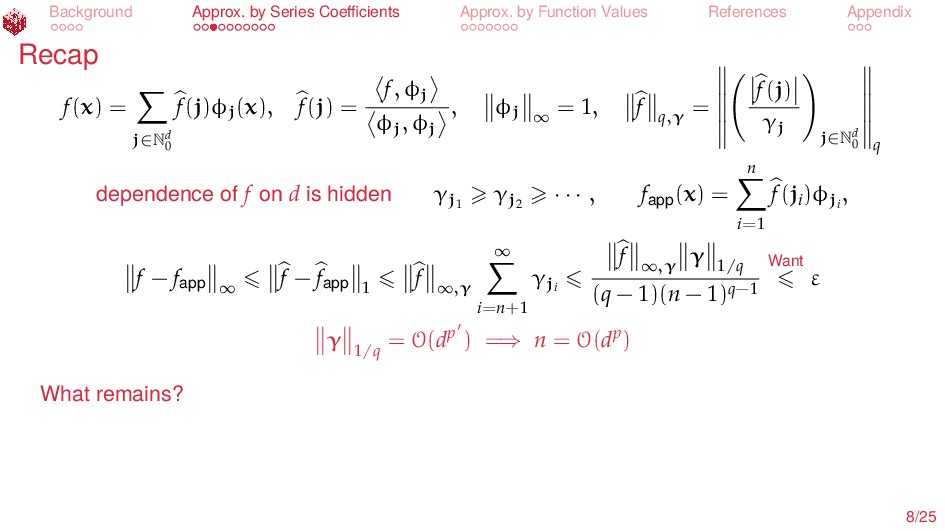
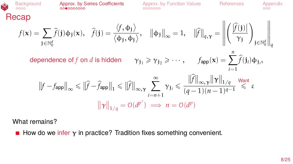
  26. Background Approx. by Series Coefficients Approx. by Function Values References

    Appendix Algorithm Using Function Values When Both γ and f ∞,γ Are Inferred Require: Γ = vector of order sizes s = vector of smoothness degrees w∗ = max k wk n0 = minimum number of wavenumbers in each coordinate C = inflation factor f = a black-box function value generator ε = positive absolute error tolerance Ensure: f − fapp ∞ ε 1: Approximate f(j) for j ∈ J := {(0, . . . , 0, j, 0 . . . , 0) : j = 1, . . . , n0 } by interpolating the function data {(xj , f(xj )) : xj = ψ(tj1 ), . . . , ψ(tjd ), j ∈ J} 2: Define w = min argmin w w∗ fj j∈J ∞,γ 3: while C fj j∈J ∞,γ j/ ∈J γj > ε do 4: Add argmin j/ ∈J γj to J 5: Approximate f(j) for j ∈ J by interpolating the function data {(xj , f(xj )) : x = ψ(tj1 ), . . . , ψ(tjd ), j ∈ J} 6: end while 7: Compute fapp = j∈J f(j)φj 18/25
  27. Background Approx. by Series Coefficients Approx. by Function Values References

    Appendix Example f(x) = exp((x2 + 1)(x3 + 1)/4) cos((x2 + 1)/2 + (x3 + 1)/2), d = 6 Bingham, D. & Surjano, S. Virtual Library of Simulation Experiments. 2013. https://www.sfu.ca/~ssurjano/. 19/25
  28. Background Approx. by Series Coefficients Approx. by Function Values References

    Appendix OTL CircuitExample Bingham, D. & Surjano, S. Virtual Library of Simulation Experiments. 2013. https://www.sfu.ca/~ssurjano/. 20/25
  29. Background Approx. by Series Coefficients Approx. by Function Values References

    Appendix Summary Functions must be nice to succeed with few function values Ideas underlying experimental design and tractability show us how to define “nice” Effect sparsity, hierarchy, heredity, and smoothness Product, order, and smoothness dependent (POSD) weighted function spaces Infer properties of f from limited data (γ, f ∞,γ , f) Must assume some structure on weights to make progress at all Design determined by wavenumbers included in approximation via van der Corput, preserves low condition number of the design matrix Gap in theory when sampling function values versus series coefficients Sample size seems to be larger than necessary Can we also infer the smoothness weights? 21/25
  30. Background Approx. by Series Coefficients Approx. by Function Values References

    Appendix Novak, E. & Woźniakowski, H. Tractability of Multivariate Problems Volume I: Linear Information. EMS Tracts in Mathematics 6 (European Mathematical Society, Zürich, 2008). Kühn, T., Sickel, W. & Ullrich, T. Approximation numbers of Sobolev embeddings—Sharp constants and tractability. J. Complexity 30, 95–116 (2014). Wu, C. F. J. & Hamada, M. Experiments: Planning, Analysis, and Parameter Design Optimization. (John Wiley & Sons, Inc., New York, 2000). Bingham, D. & Surjano, S. Virtual Library of Simulation Experiments. 2013. https://www.sfu.ca/~ssurjano/. 23/25
  31. Background Approx. by Series Coefficients Approx. by Function Values References

    Appendix In What Sense Is This Optimal? f(x) = j∈Nd 0 f(j)φj(x), f(j) = f, φj φj, φj , φj ∞ = 1, f q,γ = |f(j)| γj j∈Nd 0 q γj1 γj2 · · · , fapp(x) = n i=1 f(ji)φji , f − fapp ∞ loose f − fapp 1 tight optimal f ∞,γ ∞ i=n+1 γji For any other approximation, g, based on series coefficients, {f(j)} j∈J with |J| = n, sup h : ^ h ∞,γ = f ∞,γ ^ h(j)=f(j) ∀j∈J ^ h − ^ g 1 = f(j) − ^ g(j) j∈J 1 + sup h : ^ h ∞,γ = f ∞,γ ^ h(j) − ^ g(j) j/ ∈J 1 sup h : ^ h ∞,γ = f ∞,γ ^ h(j) j/ ∈J 1 = sup h : ^ h ∞,γ = f ∞,γ ^ h ∞,γ j/ ∈J γj f ∞,γ ∞ i=n+1 γji back 23/25
  32. Background Approx. by Series Coefficients Approx. by Function Values References

    Appendix Inferring γ from Data Given (estimates of) series coefficients, f(j) for j ∈ J := {(0, . . . , 0, j, 0 . . . , 0) : j = 1, . . . , n0}, and fixed {Γr}d r=0 , and {sj}∞ f=0 , note that f(j) j∈J ∞,γ = max j∈J |f(j)| γj = 1 Γ1 max k=1,...,d fk,max wk , fk,max := sup j=1,...,n0 |f(jek)| sj We choose wk = fk,max max f ,max , f(j) j∈J ∞,γ = max f ,max Γ1 24/25
  33. Background Approx. by Series Coefficients Approx. by Function Values References

    Appendix Tail Sum of γ The term ∞ i=n+1 γji = ∞ i=1 γji − n i=1 γji appears in the error bound. For certain γ of PSD form, we can compute the first sum on the right: j∈Nd 0 γj = u⊆1:d    ∈u w   ∞ j=1 sj   |u|   = d =1 (1 + w ssum), ssum = ∞ j=1 sj 25/25