Gregory Ditzler (with Sean Miller, Michael Valenzuela and Jerzy Rozenblit) Assistant Professor The University of Arizona Department of Electrical & Computer Engineering [email protected] uamlda.github.io April 27, 2018 ECE523: Engineering Applications of Machine Learning and Data Analytics Learning What We Don’t Care About: Regularization with Sacrificial Functions
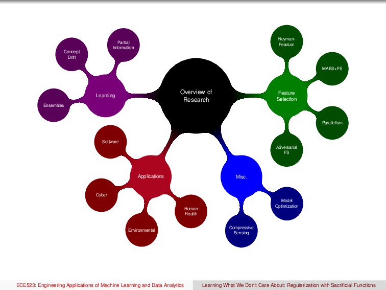
FS Misc. Model Optimization Compressive Sensing Applications Human Health Environmental Cyber Software Learning Ensembles Concept Drift Partial Information ECE523: Engineering Applications of Machine Learning and Data Analytics Learning What We Don’t Care About: Regularization with Sacrificial Functions
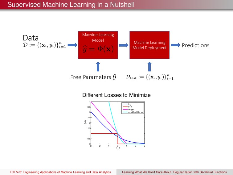
D := {(xi , yi )}n i=1 b y = (x) Dtest := {(xi , yi )}n i=1 Machine Learning Model Deployment Predictions Free Parameters ✓ Different Losses to Minimize −3 −2 −1 0 1 2 3 0 0.5 1 1.5 2 2.5 3 3.5 4 h ⋅ f L(h,f) log 0−1 hinge modified Huber ECE523: Engineering Applications of Machine Learning and Data Analytics Learning What We Don’t Care About: Regularization with Sacrificial Functions
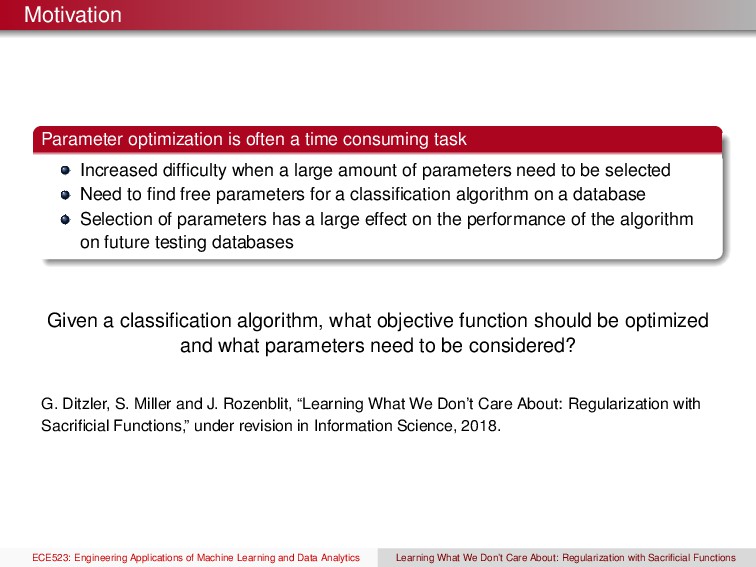
difficulty when a large amount of parameters need to be selected Need to find free parameters for a classification algorithm on a database Selection of parameters has a large effect on the performance of the algorithm on future testing databases Given a classification algorithm, what objective function should be optimized and what parameters need to be considered? G. Ditzler, S. Miller and J. Rozenblit, “Learning What We Don’t Care About: Regularization with Sacrificial Functions,” under revision in Information Science, 2018. ECE523: Engineering Applications of Machine Learning and Data Analytics Learning What We Don’t Care About: Regularization with Sacrificial Functions
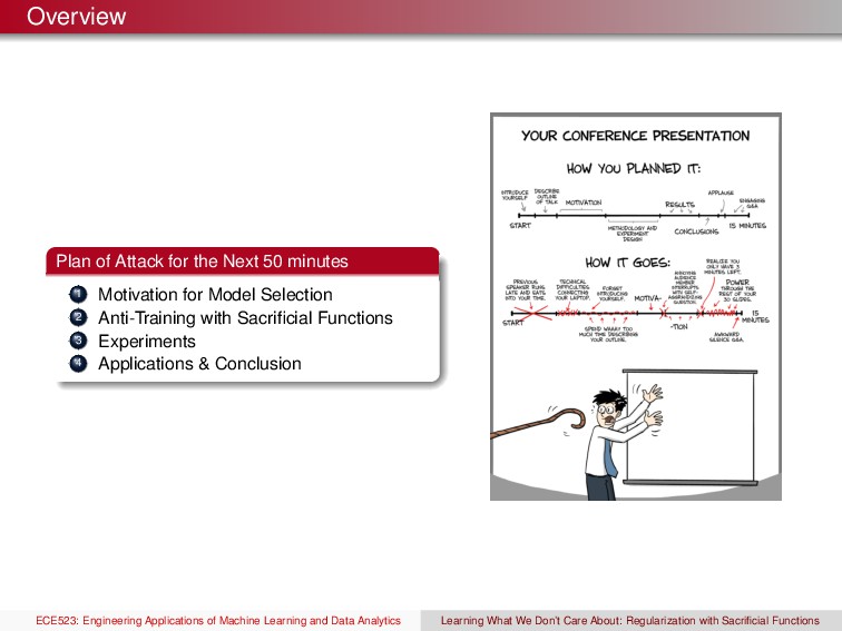
Motivation for Model Selection 2 Anti-Training with Sacrificial Functions 3 Experiments 4 Applications & Conclusion ECE523: Engineering Applications of Machine Learning and Data Analytics Learning What We Don’t Care About: Regularization with Sacrificial Functions
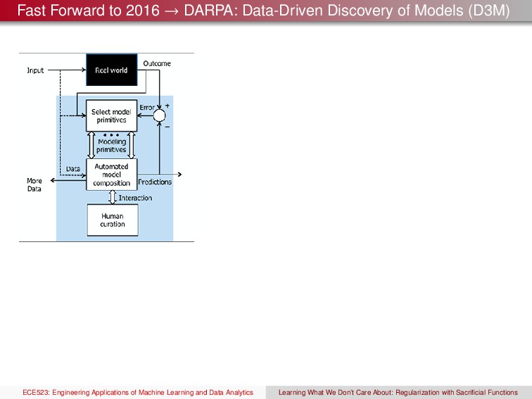
(D3M) ECE523: Engineering Applications of Machine Learning and Data Analytics Learning What We Don’t Care About: Regularization with Sacrificial Functions
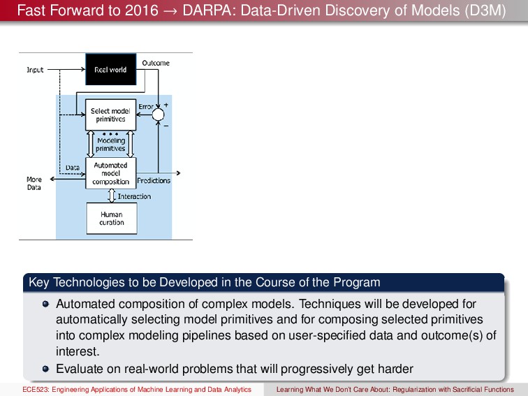
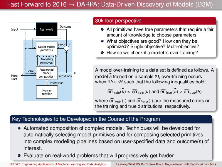
(D3M) Key Technologies to be Developed in the Course of the Program Automated composition of complex models. Techniques will be developed for automatically selecting model primitives and for composing selected primitives into complex modeling pipelines based on user-specified data and outcome(s) of interest. Evaluate on real-world problems that will progressively get harder ECE523: Engineering Applications of Machine Learning and Data Analytics Learning What We Don’t Care About: Regularization with Sacrificial Functions
(D3M) 30k foot perspective All primitives have free parameters that require a fair amount of knowledge to choose parameters What objectives are good? How can they be optimized? Single objective? Multi-objective? How do we check if a model is over-training? A model over-training to a data set is defined as follows. A model h trained on a sample D, over-training occurs when ∃h ∈ H such that the following inequalities hold: errtrain(h) < errtrain(h) and errtrue(h) > errtrue(h) where errtrain(·) and errtrue(·) are the measured errors on the training and true distributions, respectively. Key Technologies to be Developed in the Course of the Program Automated composition of complex models. Techniques will be developed for automatically selecting model primitives and for composing selected primitives into complex modeling pipelines based on user-specified data and outcome(s) of interest. Evaluate on real-world problems that will progressively get harder ECE523: Engineering Applications of Machine Learning and Data Analytics Learning What We Don’t Care About: Regularization with Sacrificial Functions
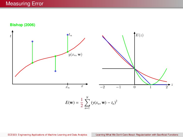
xn −2 −1 0 1 2 z E(z) E(w) = 1 2 N n=1 (y(xn , w) − tn )2 ECE523: Engineering Applications of Machine Learning and Data Analytics Learning What We Don’t Care About: Regularization with Sacrificial Functions
xn −2 −1 0 1 2 z E(z) E(w) = 1 2 N n=1 (y(xn , w) − tn )2 ECE523: Engineering Applications of Machine Learning and Data Analytics Learning What We Don’t Care About: Regularization with Sacrificial Functions
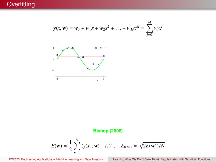
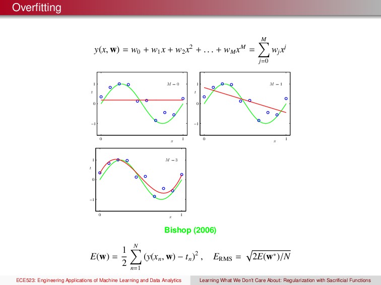
x2 + . . . + wM xM = M j=0 wj xj x t M = 0 0 1 −1 0 1 Bishop (2006) E(w) = 1 2 N n=1 (y(xn , w) − tn )2 , ERMS = 2E(w∗)/N ECE523: Engineering Applications of Machine Learning and Data Analytics Learning What We Don’t Care About: Regularization with Sacrificial Functions
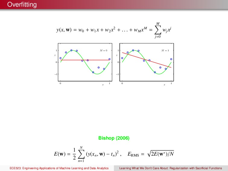
x2 + . . . + wM xM = M j=0 wj xj x t M = 0 0 1 −1 0 1 x t M = 1 0 1 −1 0 1 Bishop (2006) E(w) = 1 2 N n=1 (y(xn , w) − tn )2 , ERMS = 2E(w∗)/N ECE523: Engineering Applications of Machine Learning and Data Analytics Learning What We Don’t Care About: Regularization with Sacrificial Functions
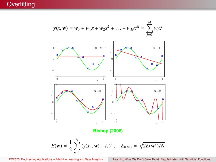
x2 + . . . + wM xM = M j=0 wj xj x t M = 0 0 1 −1 0 1 x t M = 1 0 1 −1 0 1 x t M = 3 0 1 −1 0 1 Bishop (2006) E(w) = 1 2 N n=1 (y(xn , w) − tn )2 , ERMS = 2E(w∗)/N ECE523: Engineering Applications of Machine Learning and Data Analytics Learning What We Don’t Care About: Regularization with Sacrificial Functions
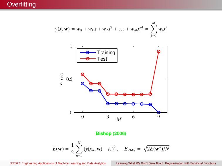
x2 + . . . + wM xM = M j=0 wj xj x t M = 0 0 1 −1 0 1 x t M = 1 0 1 −1 0 1 x t M = 3 0 1 −1 0 1 x t M = 9 0 1 −1 0 1 Bishop (2006) E(w) = 1 2 N n=1 (y(xn , w) − tn )2 , ERMS = 2E(w∗)/N ECE523: Engineering Applications of Machine Learning and Data Analytics Learning What We Don’t Care About: Regularization with Sacrificial Functions
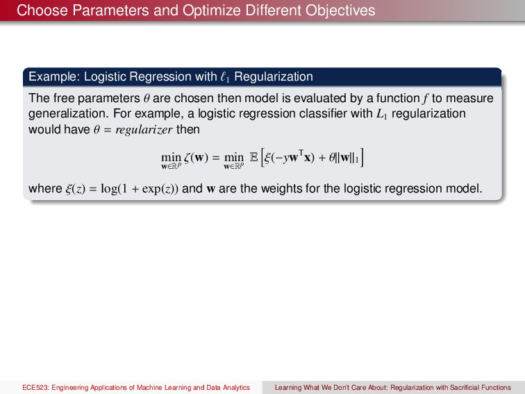
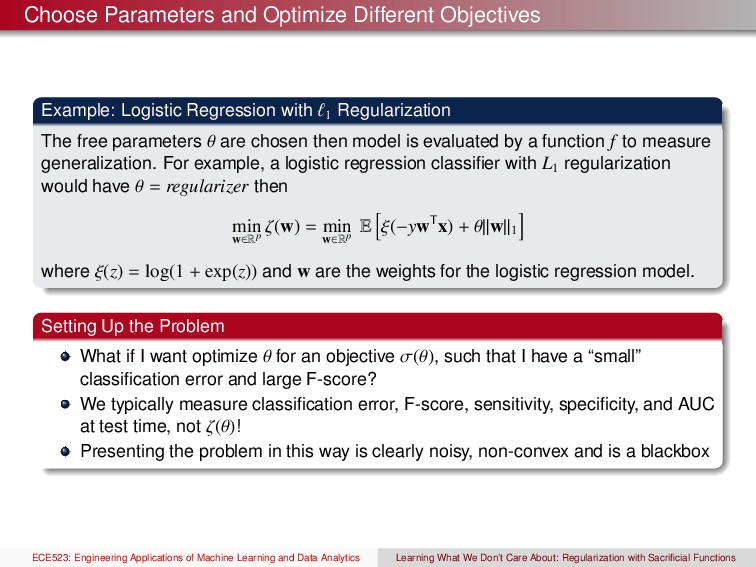
1 Regularization The free parameters θ are chosen then model is evaluated by a function f to measure generalization. For example, a logistic regression classifier with L1 regularization would have θ = regularizer then min w∈Rp ζ(w) = min w∈Rp E ξ(−ywTx) + θ w 1 where ξ(z) = log(1 + exp(z)) and w are the weights for the logistic regression model. ECE523: Engineering Applications of Machine Learning and Data Analytics Learning What We Don’t Care About: Regularization with Sacrificial Functions
1 Regularization The free parameters θ are chosen then model is evaluated by a function f to measure generalization. For example, a logistic regression classifier with L1 regularization would have θ = regularizer then min w∈Rp ζ(w) = min w∈Rp E ξ(−ywTx) + θ w 1 where ξ(z) = log(1 + exp(z)) and w are the weights for the logistic regression model. Setting Up the Problem What if I want optimize θ for an objective σ(θ), such that I have a “small” classification error and large F-score? We typically measure classification error, F-score, sensitivity, specificity, and AUC at test time, not ζ(θ)! Presenting the problem in this way is clearly noisy, non-convex and is a blackbox ECE523: Engineering Applications of Machine Learning and Data Analytics Learning What We Don’t Care About: Regularization with Sacrificial Functions
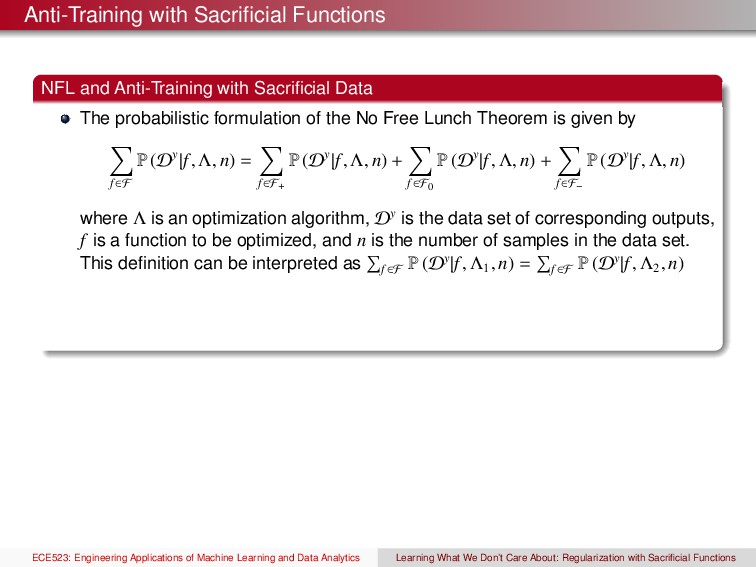
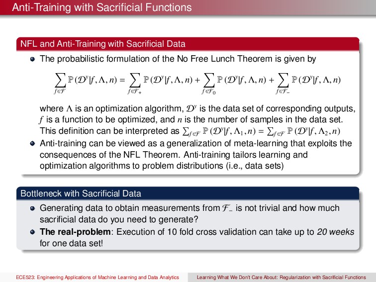
The probabilistic formulation of the No Free Lunch Theorem is given by f∈F P (Dy|f, Λ, n) = f∈F+ P (Dy|f, Λ, n) + f∈F0 P (Dy|f, Λ, n) + f∈F− P (Dy|f, Λ, n) where Λ is an optimization algorithm, Dy is the data set of corresponding outputs, f is a function to be optimized, and n is the number of samples in the data set. This definition can be interpreted as f∈F P (Dy|f, Λ1 , n) = f∈F P (Dy|f, Λ2 , n) ECE523: Engineering Applications of Machine Learning and Data Analytics Learning What We Don’t Care About: Regularization with Sacrificial Functions
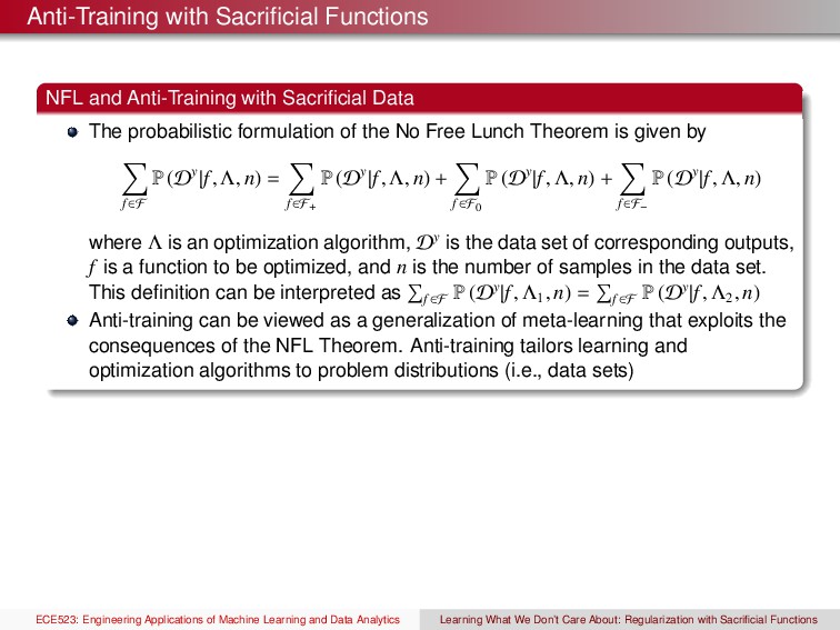
The probabilistic formulation of the No Free Lunch Theorem is given by f∈F P (Dy|f, Λ, n) = f∈F+ P (Dy|f, Λ, n) + f∈F0 P (Dy|f, Λ, n) + f∈F− P (Dy|f, Λ, n) where Λ is an optimization algorithm, Dy is the data set of corresponding outputs, f is a function to be optimized, and n is the number of samples in the data set. This definition can be interpreted as f∈F P (Dy|f, Λ1 , n) = f∈F P (Dy|f, Λ2 , n) Anti-training can be viewed as a generalization of meta-learning that exploits the consequences of the NFL Theorem. Anti-training tailors learning and optimization algorithms to problem distributions (i.e., data sets) ECE523: Engineering Applications of Machine Learning and Data Analytics Learning What We Don’t Care About: Regularization with Sacrificial Functions
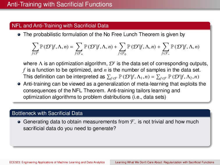
The probabilistic formulation of the No Free Lunch Theorem is given by f∈F P (Dy|f, Λ, n) = f∈F+ P (Dy|f, Λ, n) + f∈F0 P (Dy|f, Λ, n) + f∈F− P (Dy|f, Λ, n) where Λ is an optimization algorithm, Dy is the data set of corresponding outputs, f is a function to be optimized, and n is the number of samples in the data set. This definition can be interpreted as f∈F P (Dy|f, Λ1 , n) = f∈F P (Dy|f, Λ2 , n) Anti-training can be viewed as a generalization of meta-learning that exploits the consequences of the NFL Theorem. Anti-training tailors learning and optimization algorithms to problem distributions (i.e., data sets) Bottleneck with Sacrificial Data Generating data to obtain measurements from F− is not trivial and how much sacrificial data do you need to generate? ECE523: Engineering Applications of Machine Learning and Data Analytics Learning What We Don’t Care About: Regularization with Sacrificial Functions
The probabilistic formulation of the No Free Lunch Theorem is given by f∈F P (Dy|f, Λ, n) = f∈F+ P (Dy|f, Λ, n) + f∈F0 P (Dy|f, Λ, n) + f∈F− P (Dy|f, Λ, n) where Λ is an optimization algorithm, Dy is the data set of corresponding outputs, f is a function to be optimized, and n is the number of samples in the data set. This definition can be interpreted as f∈F P (Dy|f, Λ1 , n) = f∈F P (Dy|f, Λ2 , n) Anti-training can be viewed as a generalization of meta-learning that exploits the consequences of the NFL Theorem. Anti-training tailors learning and optimization algorithms to problem distributions (i.e., data sets) Bottleneck with Sacrificial Data Generating data to obtain measurements from F− is not trivial and how much sacrificial data do you need to generate? The real-problem: Execution of 10 fold cross validation can take up to 20 weeks for one data set! ECE523: Engineering Applications of Machine Learning and Data Analytics Learning What We Don’t Care About: Regularization with Sacrificial Functions
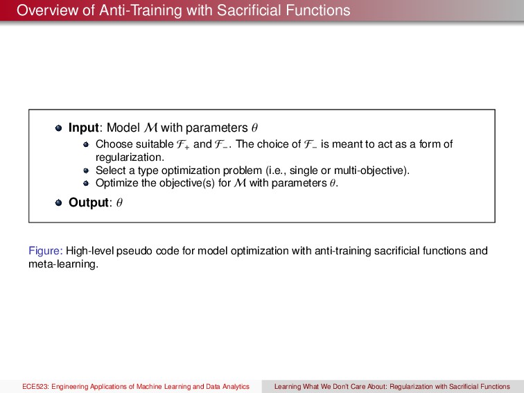
parameters θ Choose suitable F+ and F−. The choice of F− is meant to act as a form of regularization. Select a type optimization problem (i.e., single or multi-objective). Optimize the objective(s) for M with parameters θ. Output: θ Figure: High-level pseudo code for model optimization with anti-training sacrificial functions and meta-learning. ECE523: Engineering Applications of Machine Learning and Data Analytics Learning What We Don’t Care About: Regularization with Sacrificial Functions
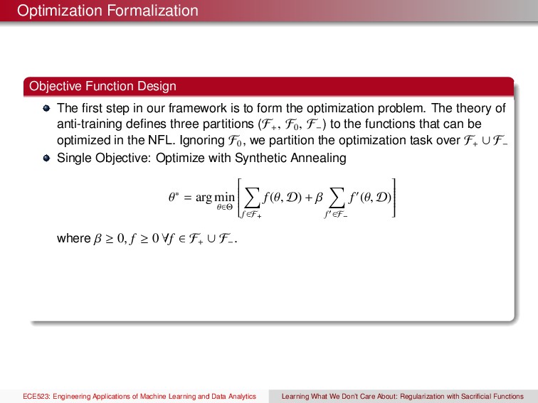
framework is to form the optimization problem. The theory of anti-training defines three partitions (F+ , F0 , F− ) to the functions that can be optimized in the NFL. Ignoring F0 , we partition the optimization task over F+ ∪ F− ECE523: Engineering Applications of Machine Learning and Data Analytics Learning What We Don’t Care About: Regularization with Sacrificial Functions
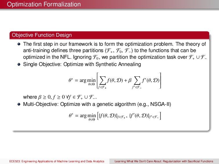
framework is to form the optimization problem. The theory of anti-training defines three partitions (F+ , F0 , F− ) to the functions that can be optimized in the NFL. Ignoring F0 , we partition the optimization task over F+ ∪ F− Single Objective: Optimize with Synthetic Annealing θ∗ = arg min θ∈Θ f∈F+ f(θ, D) + β f ∈F− f (θ, D) where β ≥ 0, f ≥ 0 ∀f ∈ F+ ∪ F− . ECE523: Engineering Applications of Machine Learning and Data Analytics Learning What We Don’t Care About: Regularization with Sacrificial Functions
framework is to form the optimization problem. The theory of anti-training defines three partitions (F+ , F0 , F− ) to the functions that can be optimized in the NFL. Ignoring F0 , we partition the optimization task over F+ ∪ F− Single Objective: Optimize with Synthetic Annealing θ∗ = arg min θ∈Θ f∈F+ f(θ, D) + β f ∈F− f (θ, D) where β ≥ 0, f ≥ 0 ∀f ∈ F+ ∪ F− . Multi-Objective: Optimize with a genetic algorithm (e.g., NSGA-II) θ∗ = arg min θ∈Θ {f(θ, D)}f∈F+ , {f (θ, D)}f ∈F− ECE523: Engineering Applications of Machine Learning and Data Analytics Learning What We Don’t Care About: Regularization with Sacrificial Functions
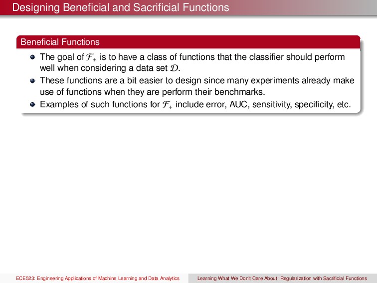
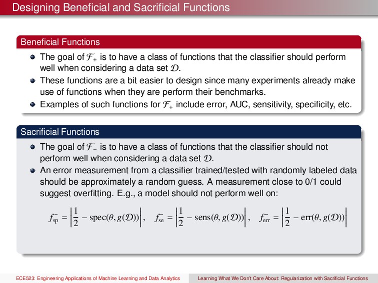
F+ is to have a class of functions that the classifier should perform well when considering a data set D. These functions are a bit easier to design since many experiments already make use of functions when they are perform their benchmarks. Examples of such functions for F+ include error, AUC, sensitivity, specificity, etc. ECE523: Engineering Applications of Machine Learning and Data Analytics Learning What We Don’t Care About: Regularization with Sacrificial Functions
F+ is to have a class of functions that the classifier should perform well when considering a data set D. These functions are a bit easier to design since many experiments already make use of functions when they are perform their benchmarks. Examples of such functions for F+ include error, AUC, sensitivity, specificity, etc. Sacrificial Functions The goal of F− is to have a class of functions that the classifier should not perform well when considering a data set D. An error measurement from a classifier trained/tested with randomly labeled data should be approximately a random guess. A measurement close to 0/1 could suggest overfitting. E.g., a model should not perform well on: f− sp = 1 2 − spec(θ, g(D)) , f− se = 1 2 − sens(θ, g(D)) , f− err = 1 2 − err(θ, g(D)) ECE523: Engineering Applications of Machine Learning and Data Analytics Learning What We Don’t Care About: Regularization with Sacrificial Functions
F+ is to have a class of functions that the classifier should perform well when considering a data set D. These functions are a bit easier to design since many experiments already make use of functions when they are perform their benchmarks. Examples of such functions for F+ include error, AUC, sensitivity, specificity, etc. Sacrificial Functions The goal of F− is to have a class of functions that the classifier should not perform well when considering a data set D. An error measurement from a classifier trained/tested with randomly labeled data should be approximately a random guess. A measurement close to 0/1 could suggest overfitting. E.g., a model should not perform well on: f− sp = 1 2 − spec(θ, g(D)) , f− se = 1 2 − sens(θ, g(D)) , f− err = 1 2 − err(θ, g(D)) Why the form of f− sp , f− se , and f− err ? arg minθ∈Θ {f+(θ, D)}f+∈F+ , {f−(θ, D)}f−∈F− ECE523: Engineering Applications of Machine Learning and Data Analytics Learning What We Don’t Care About: Regularization with Sacrificial Functions
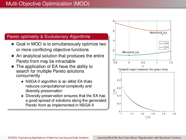
MOO is to simultaneously optimize two or more conflicting objective functions An analytical solution that produces the entire Pareto front may be intractable The application of EA have the ability to search for multiple Pareto solutions concurrently NSGA-II algorithm is an elitist EA thats reduces computational complexity and diversity preservation Diversity preservation ensures that the EA has a good spread of solutions along the generated Pareto front as implemented in NSGA-II -0.5 0 0.5 1 1.5 x Tradeoff region between the green lines 0 2 4 6 8 Minimum(f 1 (x)) Minimum(f 2 (x)) f 1 (x) f 2 (x) 1 1.1 1.2 1.3 1.4 1.5 f 1 (x) 6 6.2 6.4 6.6 6.8 7 f 2 (x) ECE523: Engineering Applications of Machine Learning and Data Analytics Learning What We Don’t Care About: Regularization with Sacrificial Functions
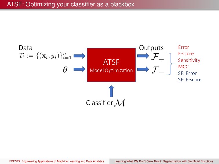
Optimization D := {(xi , yi )}n i=1 Outputs ✓ Classifier M F+ F Error F-score Sensitivity MCC SF: Error SF: F-score ECE523: Engineering Applications of Machine Learning and Data Analytics Learning What We Don’t Care About: Regularization with Sacrificial Functions
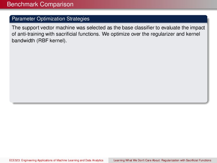
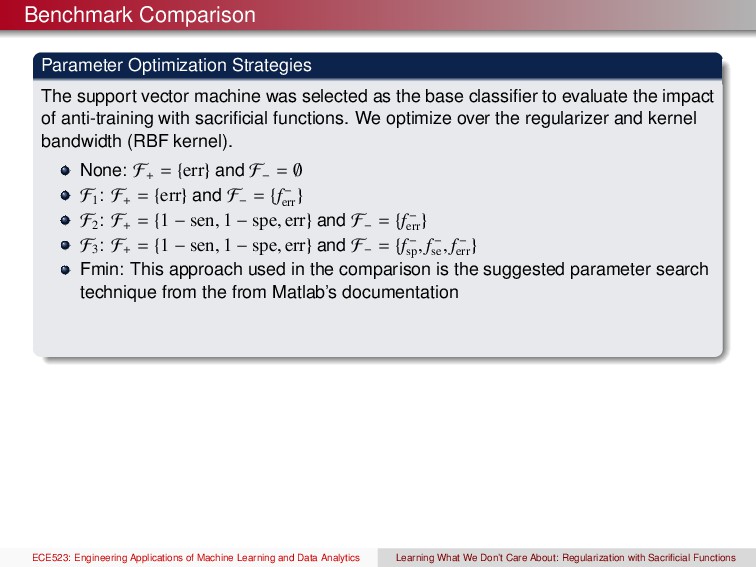
selected as the base classifier to evaluate the impact of anti-training with sacrificial functions. We optimize over the regularizer and kernel bandwidth (RBF kernel). ECE523: Engineering Applications of Machine Learning and Data Analytics Learning What We Don’t Care About: Regularization with Sacrificial Functions
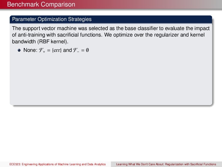
selected as the base classifier to evaluate the impact of anti-training with sacrificial functions. We optimize over the regularizer and kernel bandwidth (RBF kernel). None: F+ = {err} and F− = ∅ ECE523: Engineering Applications of Machine Learning and Data Analytics Learning What We Don’t Care About: Regularization with Sacrificial Functions
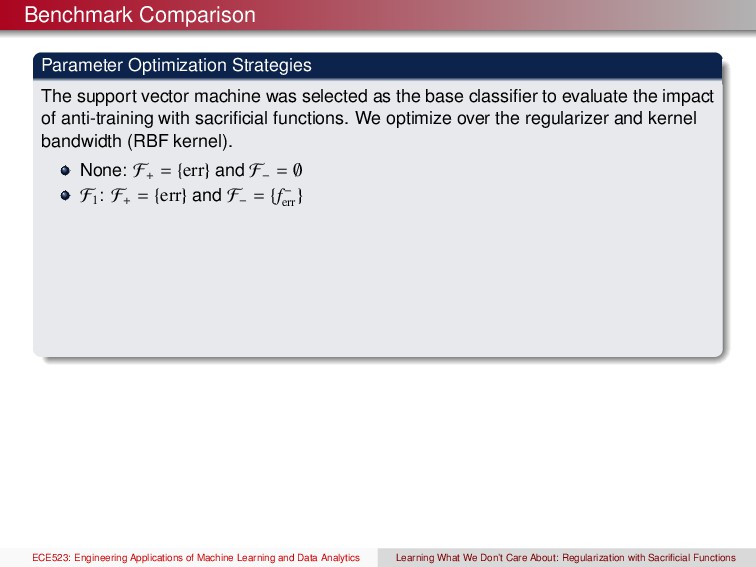
selected as the base classifier to evaluate the impact of anti-training with sacrificial functions. We optimize over the regularizer and kernel bandwidth (RBF kernel). None: F+ = {err} and F− = ∅ F1 : F+ = {err} and F− = {f− err } ECE523: Engineering Applications of Machine Learning and Data Analytics Learning What We Don’t Care About: Regularization with Sacrificial Functions
selected as the base classifier to evaluate the impact of anti-training with sacrificial functions. We optimize over the regularizer and kernel bandwidth (RBF kernel). None: F+ = {err} and F− = ∅ F1 : F+ = {err} and F− = {f− err } F2 : F+ = {1 − sen, 1 − spe, err} and F− = {f− err } ECE523: Engineering Applications of Machine Learning and Data Analytics Learning What We Don’t Care About: Regularization with Sacrificial Functions
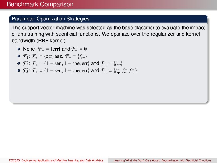
selected as the base classifier to evaluate the impact of anti-training with sacrificial functions. We optimize over the regularizer and kernel bandwidth (RBF kernel). None: F+ = {err} and F− = ∅ F1 : F+ = {err} and F− = {f− err } F2 : F+ = {1 − sen, 1 − spe, err} and F− = {f− err } F3 : F+ = {1 − sen, 1 − spe, err} and F− = {f− sp , f− se , f− err } ECE523: Engineering Applications of Machine Learning and Data Analytics Learning What We Don’t Care About: Regularization with Sacrificial Functions
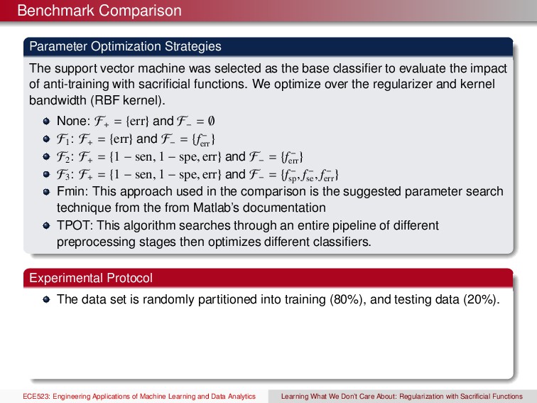
selected as the base classifier to evaluate the impact of anti-training with sacrificial functions. We optimize over the regularizer and kernel bandwidth (RBF kernel). None: F+ = {err} and F− = ∅ F1 : F+ = {err} and F− = {f− err } F2 : F+ = {1 − sen, 1 − spe, err} and F− = {f− err } F3 : F+ = {1 − sen, 1 − spe, err} and F− = {f− sp , f− se , f− err } Fmin: This approach used in the comparison is the suggested parameter search technique from the from Matlab’s documentation ECE523: Engineering Applications of Machine Learning and Data Analytics Learning What We Don’t Care About: Regularization with Sacrificial Functions
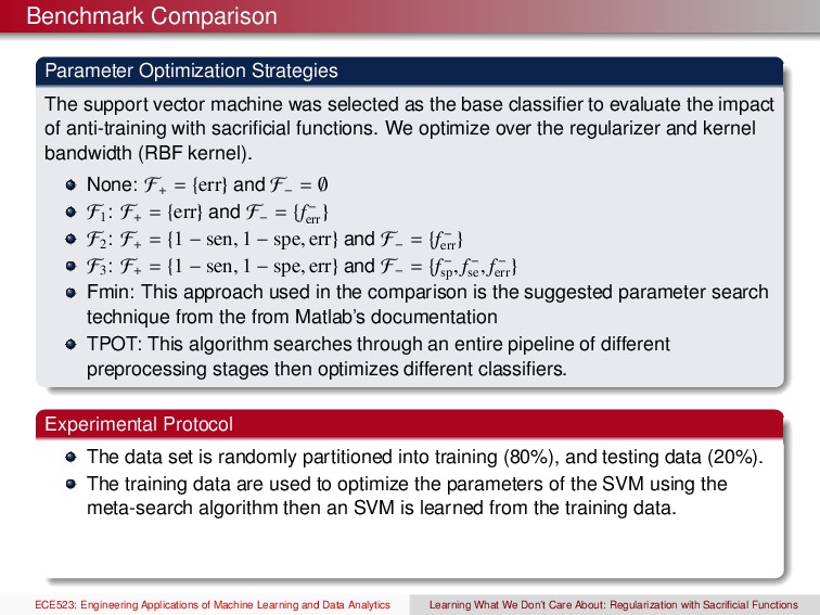
selected as the base classifier to evaluate the impact of anti-training with sacrificial functions. We optimize over the regularizer and kernel bandwidth (RBF kernel). None: F+ = {err} and F− = ∅ F1 : F+ = {err} and F− = {f− err } F2 : F+ = {1 − sen, 1 − spe, err} and F− = {f− err } F3 : F+ = {1 − sen, 1 − spe, err} and F− = {f− sp , f− se , f− err } Fmin: This approach used in the comparison is the suggested parameter search technique from the from Matlab’s documentation TPOT: This algorithm searches through an entire pipeline of different preprocessing stages then optimizes different classifiers. Experimental Protocol The data set is randomly partitioned into training (80%), and testing data (20%). ECE523: Engineering Applications of Machine Learning and Data Analytics Learning What We Don’t Care About: Regularization with Sacrificial Functions
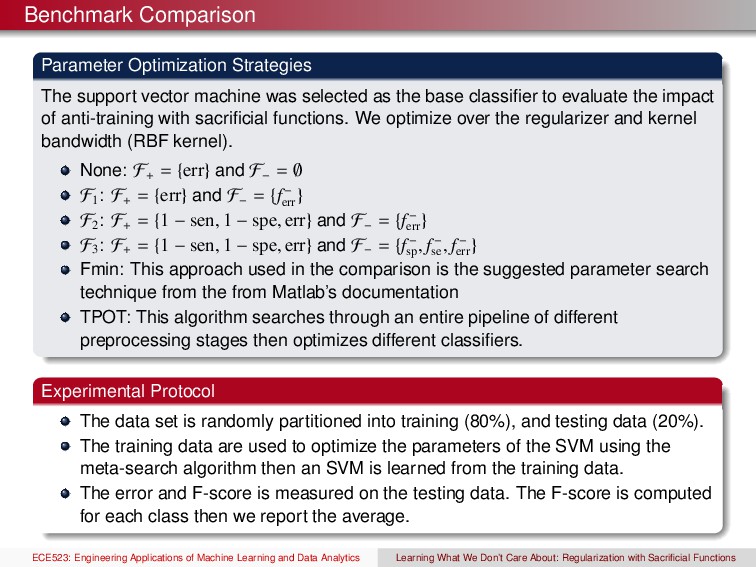
selected as the base classifier to evaluate the impact of anti-training with sacrificial functions. We optimize over the regularizer and kernel bandwidth (RBF kernel). None: F+ = {err} and F− = ∅ F1 : F+ = {err} and F− = {f− err } F2 : F+ = {1 − sen, 1 − spe, err} and F− = {f− err } F3 : F+ = {1 − sen, 1 − spe, err} and F− = {f− sp , f− se , f− err } Fmin: This approach used in the comparison is the suggested parameter search technique from the from Matlab’s documentation TPOT: This algorithm searches through an entire pipeline of different preprocessing stages then optimizes different classifiers. Experimental Protocol The data set is randomly partitioned into training (80%), and testing data (20%). The training data are used to optimize the parameters of the SVM using the meta-search algorithm then an SVM is learned from the training data. ECE523: Engineering Applications of Machine Learning and Data Analytics Learning What We Don’t Care About: Regularization with Sacrificial Functions
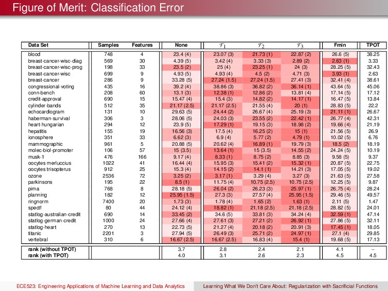
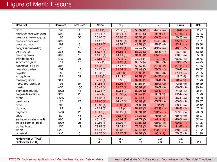
selected as the base classifier to evaluate the impact of anti-training with sacrificial functions. We optimize over the regularizer and kernel bandwidth (RBF kernel). None: F+ = {err} and F− = ∅ F1 : F+ = {err} and F− = {f− err } F2 : F+ = {1 − sen, 1 − spe, err} and F− = {f− err } F3 : F+ = {1 − sen, 1 − spe, err} and F− = {f− sp , f− se , f− err } Fmin: This approach used in the comparison is the suggested parameter search technique from the from Matlab’s documentation TPOT: This algorithm searches through an entire pipeline of different preprocessing stages then optimizes different classifiers. Experimental Protocol The data set is randomly partitioned into training (80%), and testing data (20%). The training data are used to optimize the parameters of the SVM using the meta-search algorithm then an SVM is learned from the training data. The error and F-score is measured on the testing data. The F-score is computed for each class then we report the average. ECE523: Engineering Applications of Machine Learning and Data Analytics Learning What We Don’t Care About: Regularization with Sacrificial Functions
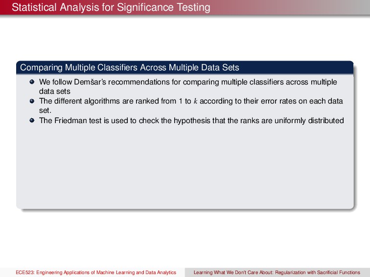
Data Sets We follow Demˇ sar’s recommendations for comparing multiple classifiers across multiple data sets The different algorithms are ranked from 1 to k according to their error rates on each data set. The Friedman test is used to check the hypothesis that the ranks are uniformly distributed ECE523: Engineering Applications of Machine Learning and Data Analytics Learning What We Don’t Care About: Regularization with Sacrificial Functions
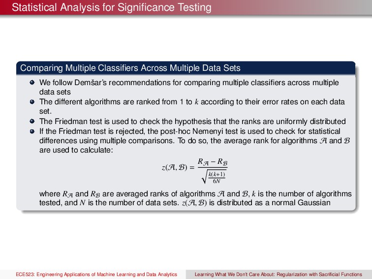
Data Sets We follow Demˇ sar’s recommendations for comparing multiple classifiers across multiple data sets The different algorithms are ranked from 1 to k according to their error rates on each data set. The Friedman test is used to check the hypothesis that the ranks are uniformly distributed If the Friedman test is rejected, the post-hoc Nemenyi test is used to check for statistical differences using multiple comparisons. To do so, the average rank for algorithms A and B are used to calculate: z(A, B) = RA − RB k(k+1) 6N where RA and RB are averaged ranks of algorithms A and B, k is the number of algorithms tested, and N is the number of data sets. z(A, B) is distributed as a normal Gaussian ECE523: Engineering Applications of Machine Learning and Data Analytics Learning What We Don’t Care About: Regularization with Sacrificial Functions
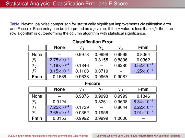
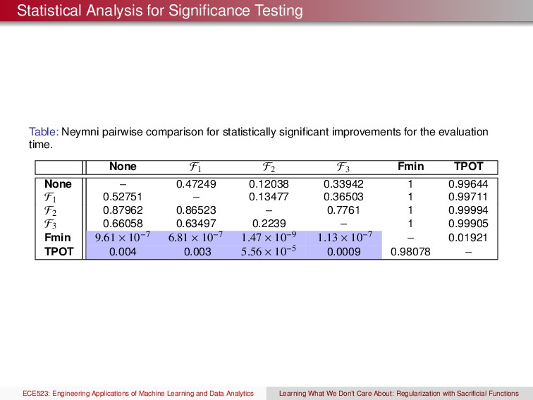
for statistically significant improvements classification error and F-score. Each entry can be interpreted as a p-value. If the p-value is less than α/4 then the row algorithm is outperforming the column algorithm with statistical significance. Classification Error None F1 F2 F3 Fmin None – 0.9973 0.9998 0.9999 0.8364 F1 2.75×10⁻³ – 0.8155 0.8896 0.0362 F2 1.19×10⁻⁴ 0.1846 – 0.6280 3.52×10⁻³ F3 3.15×10⁻⁵ 0.1103 0.3719 – 1.25×10⁻³ Fmin 0.1636 0.9638 0.9965 0.9987 – F-score None F1 F2 F3 Fmin None – 0.9876 0.9993 0.9999 0.1846 F1 0.0124 – 0.8261 0.9638 8.34×10⁻⁴ F2 7.25×10⁻⁴ 0.1739 – 0.8044 2.22×10⁻⁵ F3 2.65×10⁻⁵ 0.0362 0.1956 – 3.91×10⁻⁷ Fmin 0.8155 0.9992 0.9999 1.0000 – ECE523: Engineering Applications of Machine Learning and Data Analytics Learning What We Don’t Care About: Regularization with Sacrificial Functions
into the optimization task tends to improve upon the generalization. MOO provides a front of solutions rather than a single solutions, which provides more information to the end user. ECE523: Engineering Applications of Machine Learning and Data Analytics Learning What We Don’t Care About: Regularization with Sacrificial Functions
into the optimization task tends to improve upon the generalization. MOO provides a front of solutions rather than a single solutions, which provides more information to the end user. Current + Future Work Recent experiments with decision trees, k-NN and logistic regression confirm the findings with the support vector machine. Optimizing the MOO is still very time consuming. One approach would be to implement heuristics to speedup the parameter optimization. ECE523: Engineering Applications of Machine Learning and Data Analytics Learning What We Don’t Care About: Regularization with Sacrificial Functions
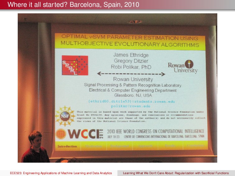
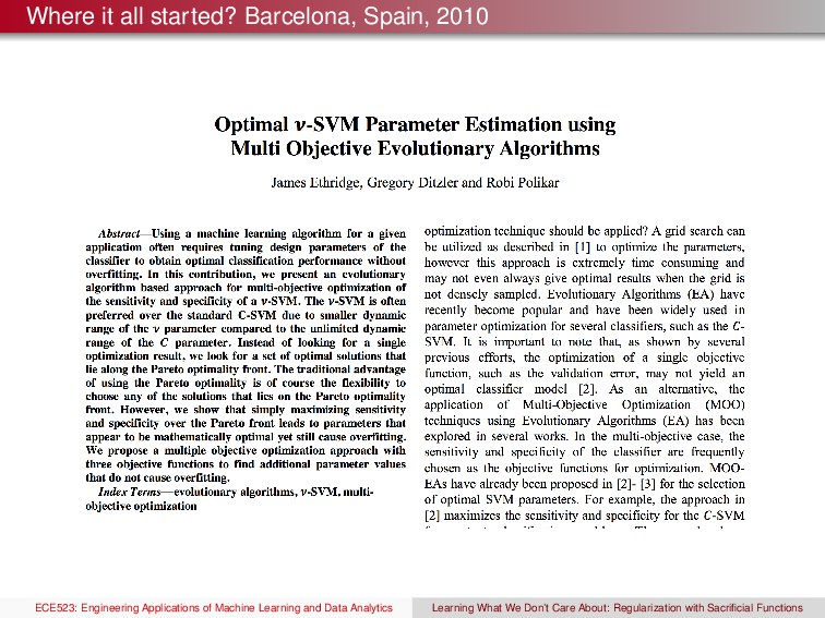
We Don’t Care About: Regularization with Sacrificial Functions,” in preparation, 2017. J. Ethridge, G. Ditzler, and R. Polikar, “Optimal ν-SVM parameter estimation using multi-objective evolutionary algorithms,” IEEE Congress on Evolutionary Computing, 2010. M. Valenzuela and J. Rozenblit, “Learning Using Anti-Training with Sacrificial Data,” Journal of Machine Learning Research, 17(24):1–42, 2016. ECE523: Engineering Applications of Machine Learning and Data Analytics Learning What We Don’t Care About: Regularization with Sacrificial Functions