with: Jean-David Benamou, Guillaume Carlier, Lenaïc Chizat, Marco Cuturi Luca Nenna, Justin Solomon, François-Xavier Vialard É C O L E N O R M A L E S U P É R I E U R E
Sliced Wasserstein projection of X to style image color statistics Y Source image after color transfer J. Rabin Wasserstein Regularization ! images, vision, graphics and machine learning, . . . • Probability distributions and histograms
Sliced Wasserstein projection of X to style image color statistics Y Source image after color transfer J. Rabin Wasserstein Regularization ! images, vision, graphics and machine learning, . . . • Probability distributions and histograms Optimal transport mean L2 mean • Optimal transport
Sliced Wasserstein projection of X to style image color statistics Y Source image after color transfer J. Rabin Wasserstein Regularization ! images, vision, graphics and machine learning, . . . • Probability distributions and histograms Optimal transport mean L2 mean • Optimal transport for Correspondence Problems auphine Vladimir G. Kim Adobe Research Suvrit Sra MIT Source Targets nce Problems G. Kim esearch Suvrit Sra MIT Targets
Probability measures. Couplings: Positive Radon measures M+(X) : P1]⇡(S) def. = ⇡(S, X) P2]⇡(S) def. = ⇡(X, S) Marginals: X = R d µ ( x ) = f ( x )d x µ = P i µ i xi ⇡ ⇧(µ, ⌫) def. = {⇡ 2 M+(X ⇥ X) ; P1]⇡ = µ, P2]⇡ = ⌫} µ(X) = 1 R f = 1 P i µi = 1 ⇡
µ, ⌫ ) def. = min ⇡ ⇢ h d p , ⇡ i = Z X⇥X d ( x, y )pd ⇡ ( x, y ) ; ⇡ 2 ⇧( µ, ⌫ ) ⇠ O(N3) Hungarian/Auction: µ = 1 N P N i =1 xi , ⌫ = 1 N P N j =1 yj Linear programming: µ = P i µ i xi , ⌫ = P j ⌫ j yj
µ, ⌫ ) def. = min ⇡ ⇢ h d p , ⇡ i = Z X⇥X d ( x, y )pd ⇡ ( x, y ) ; ⇡ 2 ⇧( µ, ⌫ ) ⇠ O(N3) Hungarian/Auction: µ = 1 N P N i =1 xi , ⌫ = 1 N P N j =1 yj Linear programming: µ = P i µ i xi , ⌫ = P j ⌫ j yj µ ⌫
|| · ||2 2. also reveal that the network simplex behaves in O ( n2 ) in our con- text, which is a major gain at the scale at which we typical work, i.e. thousands of particles. This finding is also useful for applica- tions that use EMD, where using the network simplex instead of the transport simplex can bring a significant performance increase. Our experiments also show that fixed-point precision further speeds up the computation. We observed that the value of the final trans- port cost is less accurate because of the limited precision, but that the particle pairing that produces the actual interpolation scheme remains unchanged. We used the fixed point method to generate the results presented in this paper. The results of the performance study are also of broader interest, as current EMD image retrieval or color transfer techniques rely on slower solvers [Rubner et al. 2000; Kanters et al. 2003; Morovic and Sun 2003]. 10−4 10−2 100 102 Time in seconds Network Simplex (fixed point) Network Simplex (double prec.) Transport Simplex y = α x2 y = β x3 Figure 7: Synthetic 2D examples on a Euclidean domain. Th left and right columns show the input distributions, while the cent columns show interpolations for ↵ = 1 / 4 , ↵ = 1 / 2 , and ↵ = 3 / positive. A negative side effect of this choice is that interpolatin W p p ( µ, ⌫ ) def. = min ⇡ ⇢ h d p , ⇡ i = Z X⇥X d ( x, y )pd ⇡ ( x, y ) ; ⇡ 2 ⇧( µ, ⌫ ) ⇠ O(N3) Hungarian/Auction: µ = 1 N P N i =1 xi , ⌫ = 1 N P N j =1 yj Linear programming: µ = P i µ i xi , ⌫ = P j ⌫ j yj µ ⌫
|| · ||2 2. Semi-discrete: Laguerre cells, d = || · ||2 2 . also reveal that the network simplex behaves in O ( n2 ) in our con- text, which is a major gain at the scale at which we typical work, i.e. thousands of particles. This finding is also useful for applica- tions that use EMD, where using the network simplex instead of the transport simplex can bring a significant performance increase. Our experiments also show that fixed-point precision further speeds up the computation. We observed that the value of the final trans- port cost is less accurate because of the limited precision, but that the particle pairing that produces the actual interpolation scheme remains unchanged. We used the fixed point method to generate the results presented in this paper. The results of the performance study are also of broader interest, as current EMD image retrieval or color transfer techniques rely on slower solvers [Rubner et al. 2000; Kanters et al. 2003; Morovic and Sun 2003]. 10−4 10−2 100 102 Time in seconds Network Simplex (fixed point) Network Simplex (double prec.) Transport Simplex y = α x2 y = β x3 Figure 7: Synthetic 2D examples on a Euclidean domain. Th left and right columns show the input distributions, while the cent columns show interpolations for ↵ = 1 / 4 , ↵ = 1 / 2 , and ↵ = 3 / positive. A negative side effect of this choice is that interpolatin W p p ( µ, ⌫ ) def. = min ⇡ ⇢ h d p , ⇡ i = Z X⇥X d ( x, y )pd ⇡ ( x, y ) ; ⇡ 2 ⇧( µ, ⌫ ) ⇠ O(N3) Hungarian/Auction: µ = 1 N P N i =1 xi , ⌫ = 1 N P N j =1 yj Linear programming: µ = P i µ i xi , ⌫ = P j ⌫ j yj µ ⌫ A NUMERICAL ALGORITHM FOR L2 SEMI-DISCRETE OPTIMAL TRAN Figure 9. More examples of semi-discrete optimal tra Note how the solids deform and merge to form the sphere first row, and how the branches of the star split and merge second row. A NUMERICAL ALGORITHM FOR L2 SEMI-DISCRETE OPTIMAL TRANSPORT IN 3D 21 Figure 9. More examples of semi-discrete optimal transport. Note how the solids deform and merge to form the sphere on the first row, and how the branches of the star split and merge on the second row. A NUMERICAL ALGORITHM FOR L2 SEMI-DISCRETE OPTIMAL TRANSPORT IN 3D 21 Figure 9. More examples of semi-discrete optimal transport. Note how the solids deform and merge to form the sphere on the first row, and how the branches of the star split and merge on the second row. [Levy,’15] [M´ erigot 11]
algorithms for generic c . Monge-Amp` ere/Benamou-Brenier, d = || · ||2 2. Semi-discrete: Laguerre cells, d = || · ||2 2 . also reveal that the network simplex behaves in O ( n2 ) in our con- text, which is a major gain at the scale at which we typical work, i.e. thousands of particles. This finding is also useful for applica- tions that use EMD, where using the network simplex instead of the transport simplex can bring a significant performance increase. Our experiments also show that fixed-point precision further speeds up the computation. We observed that the value of the final trans- port cost is less accurate because of the limited precision, but that the particle pairing that produces the actual interpolation scheme remains unchanged. We used the fixed point method to generate the results presented in this paper. The results of the performance study are also of broader interest, as current EMD image retrieval or color transfer techniques rely on slower solvers [Rubner et al. 2000; Kanters et al. 2003; Morovic and Sun 2003]. 10−4 10−2 100 102 Time in seconds Network Simplex (fixed point) Network Simplex (double prec.) Transport Simplex y = α x2 y = β x3 Figure 7: Synthetic 2D examples on a Euclidean domain. Th left and right columns show the input distributions, while the cent columns show interpolations for ↵ = 1 / 4 , ↵ = 1 / 2 , and ↵ = 3 / positive. A negative side effect of this choice is that interpolatin W p p ( µ, ⌫ ) def. = min ⇡ ⇢ h d p , ⇡ i = Z X⇥X d ( x, y )pd ⇡ ( x, y ) ; ⇡ 2 ⇧( µ, ⌫ ) ⇠ O(N3) Hungarian/Auction: µ = 1 N P N i =1 xi , ⌫ = 1 N P N j =1 yj Linear programming: µ = P i µ i xi , ⌫ = P j ⌫ j yj µ ⌫ A NUMERICAL ALGORITHM FOR L2 SEMI-DISCRETE OPTIMAL TRAN Figure 9. More examples of semi-discrete optimal tra Note how the solids deform and merge to form the sphere first row, and how the branches of the star split and merge second row. A NUMERICAL ALGORITHM FOR L2 SEMI-DISCRETE OPTIMAL TRANSPORT IN 3D 21 Figure 9. More examples of semi-discrete optimal transport. Note how the solids deform and merge to form the sphere on the first row, and how the branches of the star split and merge on the second row. A NUMERICAL ALGORITHM FOR L2 SEMI-DISCRETE OPTIMAL TRANSPORT IN 3D 21 Figure 9. More examples of semi-discrete optimal transport. Note how the solids deform and merge to form the sphere on the first row, and how the branches of the star split and merge on the second row. [Levy,’15] [M´ erigot 11]
e, Vialard 2015] Proposition: then WF1/2 c is a distance on M+( X ). ( ⇠, µ ) 2 M+( X ) 2 , KL( ⇠|µ ) def. = R X log ⇣ d⇠ dµ ⌘ d µ + R X (d µ d ⇠ ) If c(x, y) = log(cos(min(d(x, y), ⇡ 2 )) WFc(µ, ⌫) def. = min ⇡ hc, ⇡i + KL(P1]⇡|µ) + KL(P2]⇡|⌫) [Liereo, Mielke, Savar´ e 2015]
2015][Kondratyev, Monsaingeon, Vorotnikov, 2015] [Liereo, Mielke, Savar´ e 2015] [Chizat, Schmitzer, Peyr´ e, Vialard 2015] Proposition: then WF1/2 c is a distance on M+( X ). [Chizat, Schmitzer, P, Vialard 2015] ( ⇠, µ ) 2 M+( X ) 2 , KL( ⇠|µ ) def. = R X log ⇣ d⇠ dµ ⌘ d µ + R X (d µ d ⇠ ) If c(x, y) = log(cos(min(d(x, y), ⇡ 2 )) WFc(µ, ⌫) def. = min ⇡ hc, ⇡i + KL(P1]⇡|µ) + KL(P2]⇡|⌫) [Liereo, Mielke, Savar´ e 2015] Balanced OT Unbalanced OT
f2(P2]⇡) + "KL(⇡|⇡0) Block coordinates relaxation: max u f⇤ 1 ( u ) "he u " , Ke v " i max v f⇤ 2 ( v ) "he v " , K⇤e u " i (Iv) (Iu) Dual: (a, b) def. = (e u " , e v " ) max u,v f⇤ 1 ( u ) f⇤ 2 ( v ) "he u " , Ke v " i ⇡ ( x, y ) = a ( x ) K ( x, y ) b ( y )
f2(P2]⇡) + "KL(⇡|⇡0) Block coordinates relaxation: max u f⇤ 1 ( u ) "he u " , Ke v " i max v f⇤ 2 ( v ) "he v " , K⇤e u " i (Iv) (Iu) Proposition: Prox KL f1/"( µ ) def. = argmin ⌫f1( ⌫ ) + " KL( ⌫|µ ) the solutions of ( Iu) and ( Iv) read: a = Prox KL f1/"( Kb ) Kb b = Prox KL f2/"( K⇤a ) K⇤a Dual: (a, b) def. = (e u " , e v " ) max u,v f⇤ 1 ( u ) f⇤ 2 ( v ) "he u " , Ke v " i ⇡ ( x, y ) = a ( x ) K ( x, y ) b ( y )
! On regular grids: only convolutions! Linear time iterations. min ⇡ hdp, ⇡i + f1(P1]⇡) + f2(P2]⇡) + "KL(⇡|⇡0) Block coordinates relaxation: max u f⇤ 1 ( u ) "he u " , Ke v " i max v f⇤ 2 ( v ) "he v " , K⇤e u " i (Iv) (Iu) Proposition: Prox KL f1/"( µ ) def. = argmin ⌫f1( ⌫ ) + " KL( ⌫|µ ) the solutions of ( Iu) and ( Iv) read: a = Prox KL f1/"( Kb ) Kb b = Prox KL f2/"( K⇤a ) K⇤a Dual: (a, b) def. = (e u " , e v " ) max u,v f⇤ 1 ( u ) f⇤ 2 ( v ) "he u " , Ke v " i ⇡ ( x, y ) = a ( x ) K ( x, y ) b ( y )
W 2 (µ 2 ,µ ) µ2 W2 (µ3 ,µ ) Barycenters of measures ( µk)k: P k k = 1 If µ k = xk then µ? = P k kxk Generalizes Euclidean barycenter: µ? 2 argmin µ P k kW2 2 (µk, µ)
W 2 (µ 2 ,µ ) µ2 W2 (µ3 ,µ ) Barycenters of measures ( µk)k: P k k = 1 If µ k = xk then µ? = P k kxk Generalizes Euclidean barycenter: µ? 2 argmin µ P k kW2 2 (µk, µ)
W 2 (µ 2 ,µ ) µ2 W2 (µ3 ,µ ) Barycenters of measures ( µk)k: P k k = 1 If µ k = xk then µ? = P k kxk Generalizes Euclidean barycenter: µ2 µ1 Mc Cann’s displacement interpolation. µ? 2 argmin µ P k kW2 2 (µk, µ)
W 2 (µ 2 ,µ ) µ2 W2 (µ3 ,µ ) Barycenters of measures ( µk)k: P k k = 1 If µ k = xk then µ? = P k kxk Generalizes Euclidean barycenter: µ2 µ1 µ3 µ2 µ1 Mc Cann’s displacement interpolation. µ? 2 argmin µ P k kW2 2 (µk, µ)
W 2 (µ 2 ,µ ) µ2 W2 (µ3 ,µ ) Barycenters of measures ( µk)k: P k k = 1 If µ k = xk then µ? = P k kxk Generalizes Euclidean barycenter: µ2 µ1 µ3 µ exists and is unique. Theorem: if µ1 does not vanish on small sets, [Agueh, Carlier, 2010] (for c(x, y) = || x y ||2 ) µ2 µ1 Mc Cann’s displacement interpolation. µ? 2 argmin µ P k kW2 2 (µk, µ)
µ , i.e. choose ( ⇡0,k)k ! Sinkhorn-like algorithm [Benamou, Carlier, Cuturi, Nenna, Peyr´ e, 2015]. min (⇡k)k,µ ( X k k (hc, ⇡k i + "KL(⇡k |⇡0,k)) ; 8k, ⇡k 2 ⇧(µk, µ) )
µ , i.e. choose ( ⇡0,k)k ! Sinkhorn-like algorithm [Benamou, Carlier, Cuturi, Nenna, Peyr´ e, 2015]. [Solomon et al, SIGGRAPH 2015] min (⇡k)k,µ ( X k k (hc, ⇡k i + "KL(⇡k |⇡0,k)) ; 8k, ⇡k 2 ⇧(µk, µ) )
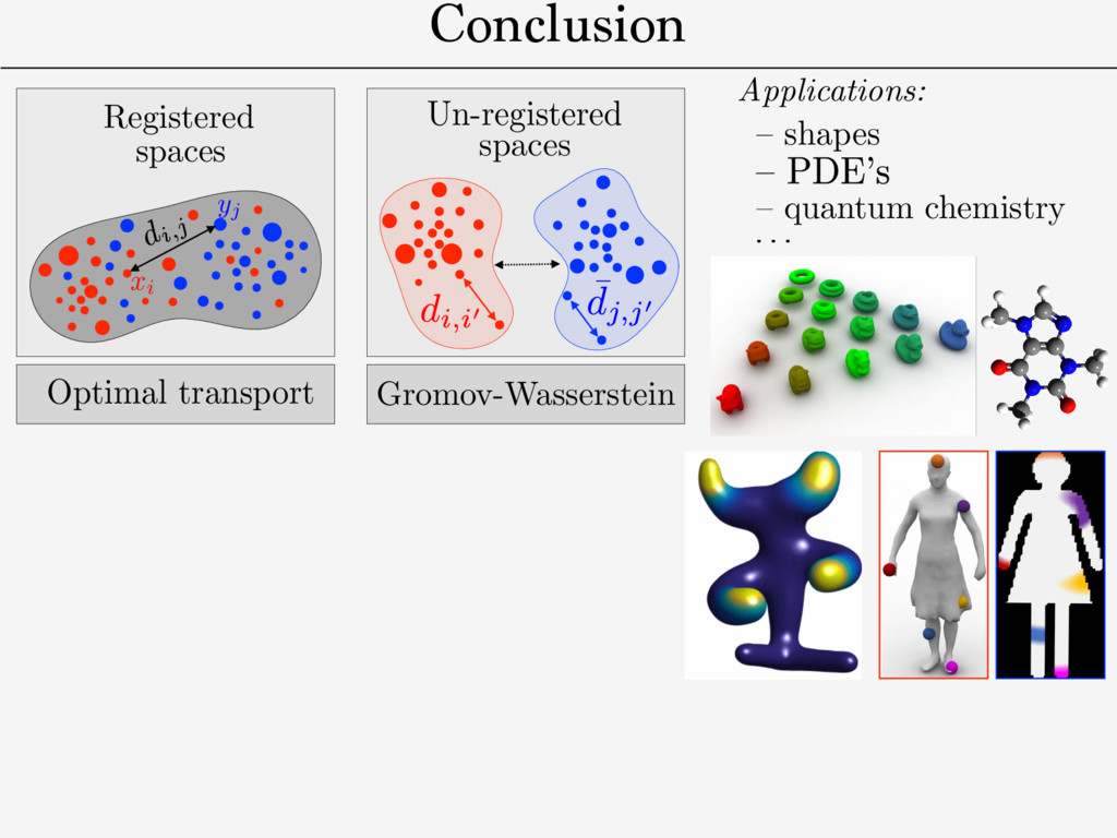
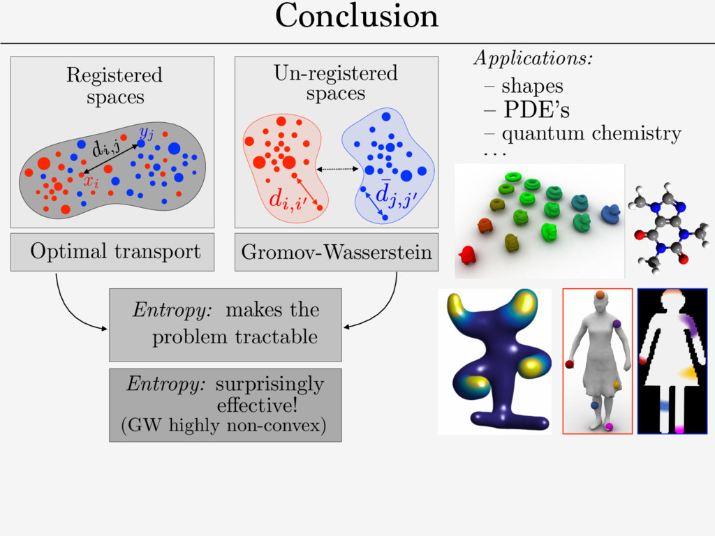
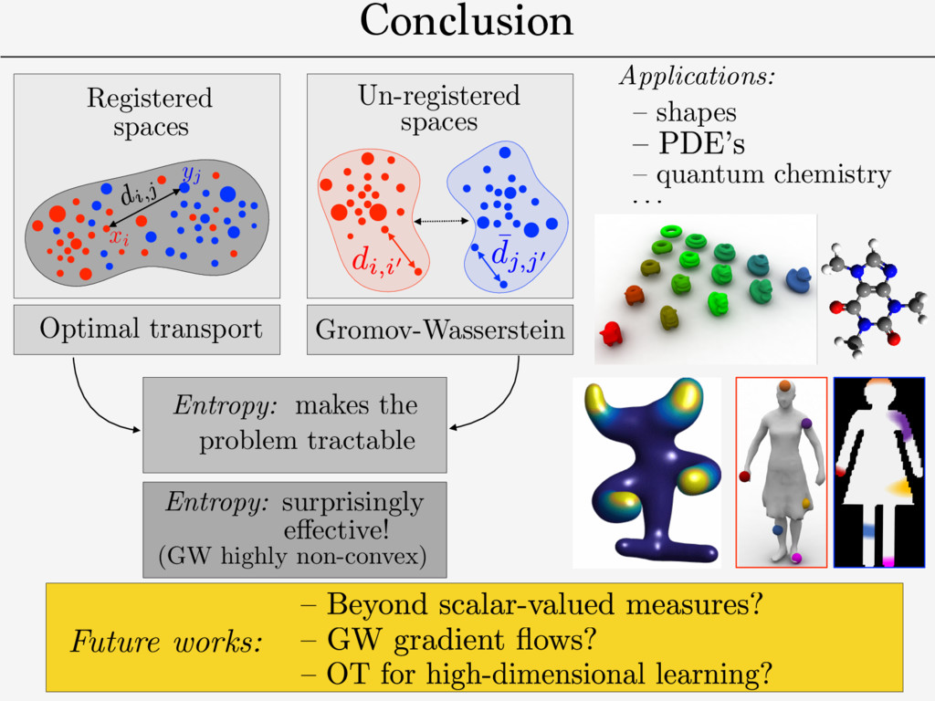
distance on mm-spaces/isometries. ! need for a fast approximate solver. ! “bending-invariant” objects recognition. ! QAP: NP-hard in general. dX ( x,x 0 ) dY (y, y0) Def. Gromov-Wasserstein distance: [Memoli 2011] [Sturm 2012] GW2 2 (dX , µ, dY , ⌫) def. = min ⇡2⇧(µ,⌫) Z X2⇥Y 2 | dX( x, x 0) dY ( y, y 0)|2d ⇡ ( x, y )d ⇡ ( x 0 , y 0) Metric-measure spaces (X, Y ): (dX , µ), (dY , ⌫)
Research Suvrit Sra MIT Source Targets Figure 1: Entropic GW can find correspondences between a source surface (left) and a surface with similar structure, a surface with shared semantic structure, a noisy 3D point cloud, an icon, and a hand drawing. Each fuzzy map was computed using the same code. In this paper, we propose a new correspondence algorithm that minimizes distortion of long- and short-range distances alike. We study an entropically-regularized version of the Gromov-Wasserstein (GW) mapping objective function from [M´ emoli 2011] measuring the distortion of geodesic distances. The optimizer is a probabilistic matching expressed as a “fuzzy” correspondence matrix in the style of [Kim et al. 2012; Solomon et al. 2012]; we control sharpness of the correspondence via the weight of the entropic regularizer. 0 0.02 0.04 0 0.02 0 0.02 Teddies Humans Four-legged Armadillo Figure 15: MDS embedding of four classes from SHREC dataset. 0 0.5 1 0 0.5 1 1 5 10 15 20 25 30 35 40 45 PCA 1 PCA 2 Figure 16: Recovery of galloping horse sequence. 0 is the base shape) as a feature vector for shape i. We reproduce the result presented in the work of Rustamov et al., recovering the circular structure of meshes from a galloping horse animation sequence (Figure 16). Unlike Rustamov et al., however, our method does not require ground truth maps between shapes as input. 5.2 Supervised Matching An important feature of a matching tool is the ability to incorporate user input, e.g. ground truth matches of points or regions. In the GWα framework, one way to enforce these constraints is to provide a stencil S specifying a sparsity pattern for the map Γ. Incorporating Figure 18: Mapping a set of 185 images onto a two shapes while preserving color similarity. (Images from Flickr public domain collection.) Rn0×n0 + and D ∈ Rn×n + we are given symmetric weight matrices W0 ∈ Rn0×n0 + and W ∈ Rn×n + . We could solve a weighted version of the GWα matching problem (3) that prioritizes maps preserving distances corresponding to large W values: min Γ∈M ijkℓ (D0ij −Dkℓ )2ΓikΓjℓW0ijWjℓµ0iµ0jµkµℓ . (8) For instance, (W0, W) might contain confidence values expressing the quality of the entries of (D0, D). Or, W0, W could take values in {ε, 1} reducing the weight of distances that are unknown or do not need to be preserved by Γ. Following the same simplifications as §3.1, we can optimize this objective by minimizing ⟨Γ, ΛW (Γ)⟩, where ΛW (Γ) := 1 2 [D∧2 0 ⊗ W0][[µ0 ]]Γ[[µ]]W − [D0 ⊗ W0][[µ0 ]]Γ[[µ]][D ⊗ W] + 1 2 W0[[µ0 ]]Γ[[µ]][D∧2 ⊗ W] Use T to define registration between: Colors distribution Shape Shape Shape
Research Suvrit Sra MIT Source Targets Figure 1: Entropic GW can find correspondences between a source surface (left) and a surface with similar structure, a surface with shared semantic structure, a noisy 3D point cloud, an icon, and a hand drawing. Each fuzzy map was computed using the same code. In this paper, we propose a new correspondence algorithm that minimizes distortion of long- and short-range distances alike. We study an entropically-regularized version of the Gromov-Wasserstein (GW) mapping objective function from [M´ emoli 2011] measuring the distortion of geodesic distances. The optimizer is a probabilistic matching expressed as a “fuzzy” correspondence matrix in the style of [Kim et al. 2012; Solomon et al. 2012]; we control sharpness of the correspondence via the weight of the entropic regularizer. 0 0.02 0.04 0 0.02 0 0.02 Teddies Humans Four-legged Armadillo Figure 15: MDS embedding of four classes from SHREC dataset. 0 0.5 1 0 0.5 1 1 5 10 15 20 25 30 35 40 45 PCA 1 PCA 2 Figure 16: Recovery of galloping horse sequence. 0 is the base shape) as a feature vector for shape i. We reproduce the result presented in the work of Rustamov et al., recovering the circular structure of meshes from a galloping horse animation sequence (Figure 16). Unlike Rustamov et al., however, our method does not require ground truth maps between shapes as input. 5.2 Supervised Matching An important feature of a matching tool is the ability to incorporate user input, e.g. ground truth matches of points or regions. In the GWα framework, one way to enforce these constraints is to provide a stencil S specifying a sparsity pattern for the map Γ. Incorporating Figure 18: Mapping a set of 185 images onto a two shapes while preserving color similarity. (Images from Flickr public domain collection.) Rn0×n0 + and D ∈ Rn×n + we are given symmetric weight matrices W0 ∈ Rn0×n0 + and W ∈ Rn×n + . We could solve a weighted version of the GWα matching problem (3) that prioritizes maps preserving distances corresponding to large W values: min Γ∈M ijkℓ (D0ij −Dkℓ )2ΓikΓjℓW0ijWjℓµ0iµ0jµkµℓ . (8) For instance, (W0, W) might contain confidence values expressing the quality of the entries of (D0, D). Or, W0, W could take values in {ε, 1} reducing the weight of distances that are unknown or do not need to be preserved by Γ. Following the same simplifications as §3.1, we can optimize this objective by minimizing ⟨Γ, ΛW (Γ)⟩, where ΛW (Γ) := 1 2 [D∧2 0 ⊗ W0][[µ0 ]]Γ[[µ]]W − [D0 ⊗ W0][[µ0 ]]Γ[[µ]][D ⊗ W] + 1 2 W0[[µ0 ]]Γ[[µ]][D∧2 ⊗ W] 0 0.02 0.04 0 0.02 0 0.02 Te Hu Fo Ar Figure 1: The database that has been used, divide MDS in 3-D Use T to define registration between: Colors distribution Shape Shape Shape Geodesic distances GW distances MDS Vizualization Shapes (Xs)s 0 0.02 0.04 0 0.02 0 0.02 Teddies Humans Four-legged Armadillo Figure 15: MDS embedding of four classes from SHREC dataset. 0 0.5 1 1 5 10 15 20 25 30 35 40 45 PCA 2 Figure 18: Mapping a set of 185 images onto a two shapes while preserving color similarity. (Images from Flickr public domain collection.) Rn0×n0 + and D ∈ Rn×n + we are given symmetric weight matrices W0 ∈ Rn0×n0 + and W ∈ Rn×n + . We could solve a weighted version of the GWα matching problem (3) that prioritizes maps preserving distances corresponding to large W values: MDS in 2-D
– quantum chemistry – shapes Entropic Metric Alignment for Corresponde Justin Solomon∗ MIT Gabriel Peyr´ e CNRS & Univ. Paris-Dauphine Vladimi Adobe R Abstract Many shape and image processing tools rely on computation of cor- respondences between geometric domains. Efficient methods that stably extract “soft” matches in the presence of diverse geometric structures have proven to be valuable for shape retrieval and transfer of labels or semantic information. With these applications in mind, we present an algorithm for probabilistic correspondence that opti- mizes an entropy-regularized Gromov-Wasserstein (GW) objective. Built upon recent developments in numerical optimal transportation, our algorithm is compact, provably convergent, and applicable to any geometric domain expressible as a metric measure matrix. We Source Figure 1: Entropic G surface (left) and a s shared semantic stru ic Metric Alignment for Correspondence Problems n∗ Gabriel Peyr´ e CNRS & Univ. Paris-Dauphine Vladimir G. Kim Adobe Research Suvrit Sra MIT ng tools rely on computation of cor- c domains. Efficient methods that the presence of diverse geometric able for shape retrieval and transfer n. With these applications in mind, babilistic correspondence that opti- omov-Wasserstein (GW) objective. n numerical optimal transportation, ably convergent, and applicable to le as a metric measure matrix. We Source Targets Figure 1: Entropic GW can find correspondences between surface (left) and a surface with similar structure, a surf shared semantic structure, a noisy 3D point cloud, an ico Conclusion
– quantum chemistry – shapes Entropic Metric Alignment for Corresponde Justin Solomon∗ MIT Gabriel Peyr´ e CNRS & Univ. Paris-Dauphine Vladimi Adobe R Abstract Many shape and image processing tools rely on computation of cor- respondences between geometric domains. Efficient methods that stably extract “soft” matches in the presence of diverse geometric structures have proven to be valuable for shape retrieval and transfer of labels or semantic information. With these applications in mind, we present an algorithm for probabilistic correspondence that opti- mizes an entropy-regularized Gromov-Wasserstein (GW) objective. Built upon recent developments in numerical optimal transportation, our algorithm is compact, provably convergent, and applicable to any geometric domain expressible as a metric measure matrix. We Source Figure 1: Entropic G surface (left) and a s shared semantic stru ic Metric Alignment for Correspondence Problems n∗ Gabriel Peyr´ e CNRS & Univ. Paris-Dauphine Vladimir G. Kim Adobe Research Suvrit Sra MIT ng tools rely on computation of cor- c domains. Efficient methods that the presence of diverse geometric able for shape retrieval and transfer n. With these applications in mind, babilistic correspondence that opti- omov-Wasserstein (GW) objective. n numerical optimal transportation, ably convergent, and applicable to le as a metric measure matrix. We Source Targets Figure 1: Entropic GW can find correspondences between surface (left) and a surface with similar structure, a surf shared semantic structure, a noisy 3D point cloud, an ico Conclusion
makes the problem tractable e↵ective! Entropy: surprisingly (GW highly non-convex) Applications: – quantum chemistry – shapes Entropic Metric Alignment for Corresponde Justin Solomon∗ MIT Gabriel Peyr´ e CNRS & Univ. Paris-Dauphine Vladimi Adobe R Abstract Many shape and image processing tools rely on computation of cor- respondences between geometric domains. Efficient methods that stably extract “soft” matches in the presence of diverse geometric structures have proven to be valuable for shape retrieval and transfer of labels or semantic information. With these applications in mind, we present an algorithm for probabilistic correspondence that opti- mizes an entropy-regularized Gromov-Wasserstein (GW) objective. Built upon recent developments in numerical optimal transportation, our algorithm is compact, provably convergent, and applicable to any geometric domain expressible as a metric measure matrix. We Source Figure 1: Entropic G surface (left) and a s shared semantic stru ic Metric Alignment for Correspondence Problems n∗ Gabriel Peyr´ e CNRS & Univ. Paris-Dauphine Vladimir G. Kim Adobe Research Suvrit Sra MIT ng tools rely on computation of cor- c domains. Efficient methods that the presence of diverse geometric able for shape retrieval and transfer n. With these applications in mind, babilistic correspondence that opti- omov-Wasserstein (GW) objective. n numerical optimal transportation, ably convergent, and applicable to le as a metric measure matrix. We Source Targets Figure 1: Entropic GW can find correspondences between surface (left) and a surface with similar structure, a surf shared semantic structure, a noisy 3D point cloud, an ico Conclusion
makes the problem tractable e↵ective! Entropy: surprisingly (GW highly non-convex) Applications: – quantum chemistry – shapes Entropic Metric Alignment for Corresponde Justin Solomon∗ MIT Gabriel Peyr´ e CNRS & Univ. Paris-Dauphine Vladimi Adobe R Abstract Many shape and image processing tools rely on computation of cor- respondences between geometric domains. Efficient methods that stably extract “soft” matches in the presence of diverse geometric structures have proven to be valuable for shape retrieval and transfer of labels or semantic information. With these applications in mind, we present an algorithm for probabilistic correspondence that opti- mizes an entropy-regularized Gromov-Wasserstein (GW) objective. Built upon recent developments in numerical optimal transportation, our algorithm is compact, provably convergent, and applicable to any geometric domain expressible as a metric measure matrix. We Source Figure 1: Entropic G surface (left) and a s shared semantic stru ic Metric Alignment for Correspondence Problems n∗ Gabriel Peyr´ e CNRS & Univ. Paris-Dauphine Vladimir G. Kim Adobe Research Suvrit Sra MIT ng tools rely on computation of cor- c domains. Efficient methods that the presence of diverse geometric able for shape retrieval and transfer n. With these applications in mind, babilistic correspondence that opti- omov-Wasserstein (GW) objective. n numerical optimal transportation, ably convergent, and applicable to le as a metric measure matrix. We Source Targets Figure 1: Entropic GW can find correspondences between surface (left) and a surface with similar structure, a surf shared semantic structure, a noisy 3D point cloud, an ico Future works: Conclusion
![Optimal Transport Optimal transport: [Kantorovitch 1942] W p p (](https://files.speakerdeck.com/presentations/ba0a345b9a594f9294488d4cb2ec4ac8/slide_7.jpg)
![Optimal Transport Optimal transport: [Kantorovitch 1942] W p p (](https://files.speakerdeck.com/presentations/ba0a345b9a594f9294488d4cb2ec4ac8/slide_8.jpg)
![Optimal Transport Optimal transport: [Kantorovitch 1942] W p p (](https://files.speakerdeck.com/presentations/ba0a345b9a594f9294488d4cb2ec4ac8/slide_9.jpg)
![Optimal Transport Optimal transport: [Kantorovitch 1942] W p p (](https://files.speakerdeck.com/presentations/ba0a345b9a594f9294488d4cb2ec4ac8/slide_10.jpg)
![Optimal Transport Optimal transport: [Kantorovitch 1942] Monge-Amp` ere/Benamou-Brenier, d =](https://files.speakerdeck.com/presentations/ba0a345b9a594f9294488d4cb2ec4ac8/slide_11.jpg)
![Optimal Transport Optimal transport: [Kantorovitch 1942] Monge-Amp` ere/Benamou-Brenier, d =](https://files.speakerdeck.com/presentations/ba0a345b9a594f9294488d4cb2ec4ac8/slide_12.jpg)
![Optimal Transport Optimal transport: [Kantorovitch 1942] Need for fast approximate](https://files.speakerdeck.com/presentations/ba0a345b9a594f9294488d4cb2ec4ac8/slide_13.jpg)
![Unbalanced Transport [Liereo, Mielke, Savar´ e 2015] [Chizat, Schmitzer, Peyr´](https://files.speakerdeck.com/presentations/ba0a345b9a594f9294488d4cb2ec4ac8/slide_15.jpg)
![Wasserstein Gradient Flows Implicit Euler step: [Jordan, Kinderlehrer, Otto 1998]](https://files.speakerdeck.com/presentations/ba0a345b9a594f9294488d4cb2ec4ac8/slide_17.jpg)
![Wasserstein Gradient Flows Implicit Euler step: [Jordan, Kinderlehrer, Otto 1998]](https://files.speakerdeck.com/presentations/ba0a345b9a594f9294488d4cb2ec4ac8/slide_18.jpg)
![Wasserstein Gradient Flows Implicit Euler step: [Jordan, Kinderlehrer, Otto 1998]](https://files.speakerdeck.com/presentations/ba0a345b9a594f9294488d4cb2ec4ac8/slide_19.jpg)
![Wasserstein Gradient Flows Implicit Euler step: [Jordan, Kinderlehrer, Otto 1998]](https://files.speakerdeck.com/presentations/ba0a345b9a594f9294488d4cb2ec4ac8/slide_20.jpg)
![Wasserstein Gradient Flows Implicit Euler step: [Jordan, Kinderlehrer, Otto 1998]](https://files.speakerdeck.com/presentations/ba0a345b9a594f9294488d4cb2ec4ac8/slide_21.jpg)
![Dykstra-like Iterations Primal: min ⇡ hdp, ⇡i + f1(P1]⇡) +](https://files.speakerdeck.com/presentations/ba0a345b9a594f9294488d4cb2ec4ac8/slide_28.jpg)
![Dykstra-like Iterations Primal: min ⇡ hdp, ⇡i + f1(P1]⇡) +](https://files.speakerdeck.com/presentations/ba0a345b9a594f9294488d4cb2ec4ac8/slide_29.jpg)
![Dykstra-like Iterations Primal: min ⇡ hdp, ⇡i + f1(P1]⇡) +](https://files.speakerdeck.com/presentations/ba0a345b9a594f9294488d4cb2ec4ac8/slide_30.jpg)
![Dykstra-like Iterations Primal: min ⇡ hdp, ⇡i + f1(P1]⇡) +](https://files.speakerdeck.com/presentations/ba0a345b9a594f9294488d4cb2ec4ac8/slide_31.jpg)