Joint modelling of longitudinal and time-to-event data with R

A half-day workshop at the SAM 2017 Conference

Transcript

1. Introduction Univariate joint models Competing risks Multivariate data Summary References Joint modelling of longitudinal and time-to-event data with R Graeme L. Hickey Department of Biostatistics, University of Liverpool, UK graeme.hickey@liverpool.ac.uk 5th July 2017 1/98
2. Introduction Univariate joint models Competing risks Multivariate data Summary References An MRC funded workshop 2/98
3. Introduction Univariate joint models Competing risks Multivariate data Summary References Timetable Time What Who 0900 – 0920 Introduction G. L. Hickey 0920 – 0940 Univariate joint models P. Philipson 0940 – 1000 Competing risks R. Kolamunnage-Dona 1000 – 1025 Multivariate outcomes G. L. Hickey 1025 – 1030 Summary G. L. Hickey 1030 – 1045 Tea and coffee break 1045 – 1100 Overview of R packages G. L. Hickey 1100 – 1230 Practical worksheet & problems sheet 1230 – 1300 Lunch 3/98
4. Introduction Univariate joint models Competing risks Multivariate data Summary References Practical information References are given in the bibliograpy (slide 95 – onwards) Time for questions during the break and lunch sessions1 1Please find myself, Ruwanthi, Pete, Maria, or Andrea 4/98
5. Introduction Univariate joint models Competing risks Multivariate data Summary References Introduction 5/98
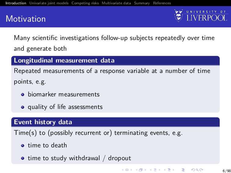
6. Introduction Univariate joint models Competing risks Multivariate data Summary References Motivation Many scientific investigations follow-up subjects repeatedly over time and generate both Longitudinal measurement data Repeated measurements of a response variable at a number of time points, e.g. biomarker measurements quality of life assessments Event history data Time(s) to (possibly recurrent or) terminating events, e.g. time to death time to study withdrawal / dropout 6/98
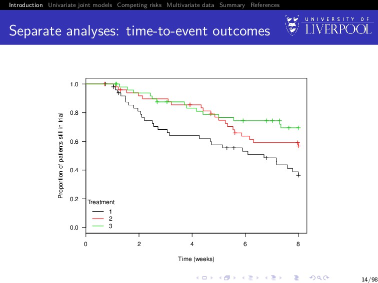
7. Introduction Univariate joint models Competing risks Multivariate data Summary References Schizophrenia trial data A placebo-controlled randomized clinical trial of drug treatments for schizophrenia (Henderson et al. 2000) In the original trial there were three treatment arms: placebo, standard, and novel compound (subdivided into 4 dosages) We will analyse a sample of 150 patients (50 patients per treatment arm) 7/98
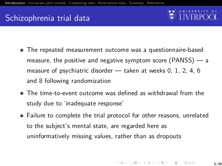
8. Introduction Univariate joint models Competing risks Multivariate data Summary References Schizophrenia trial data The repeated measurement outcome was a questionnaire-based measure, the positive and negative symptom score (PANSS) — a measure of psychiatric disorder — taken at weeks 0, 1, 2, 4, 6 and 8 following randomization The time-to-event outcome was defined as withdrawal from the study due to ‘inadequate response’ Failure to complete the trial protocol for other reasons, unrelated to the subject’s mental state, are regarded here as uninformatively missing values, rather than as dropouts 8/98
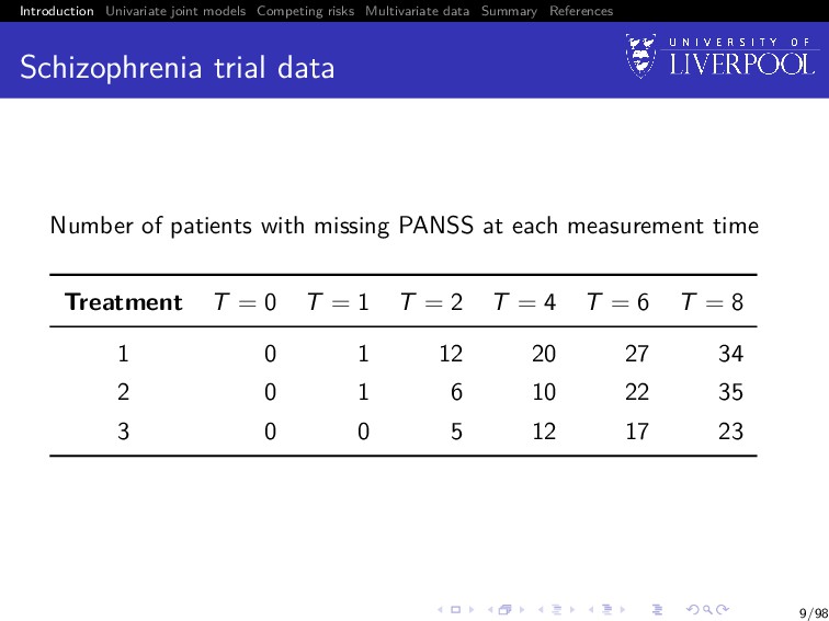
9. Introduction Univariate joint models Competing risks Multivariate data Summary References Schizophrenia trial data Number of patients with missing PANSS at each measurement time Treatment T = 0 T = 1 T = 2 T = 4 T = 6 T = 8 1 0 1 12 20 27 34 2 0 1 6 10 22 35 3 0 0 5 12 17 23 9/98
10. Introduction Univariate joint models Competing risks Multivariate data Summary References Focus Depending of the focus of the research question, we might use either Separate analyses of one or more of the outcomes Joint analysis of the different outcomes 10/98
11. Introduction Univariate joint models Competing risks Multivariate data Summary References Separate analyses Is the average PANSS score trajectory different between treatment groups? Does patient dropout differ between treatment group? 11/98
12. Introduction Univariate joint models Competing risks Multivariate data Summary References Separate analyses: longitudinal outcomes 20 40 60 80 100 0 1 2 4 6 8 Time (weeks) PANSS Treatment 1 2 3 12/98
13. Introduction Univariate joint models Competing risks Multivariate data Summary References Separate analyses: longitudinal outcomes Linear mixed effects model with treatment Xi ∈ {1, 2, 3} Yi (t) = (β0 + bi0) + (β1 + bi1)t + β2I(Xi = 2)t + β3I(Xi = 3)t + εi (t) (bi0, bi1) ∼ N2(0, D) εi (t) i.i.d. ∼ N(0, σ2) 13/98
14. Introduction Univariate joint models Competing risks Multivariate data Summary References Separate analyses: longitudinal outcomes Linear mixed effects model with treatment Xi ∈ {1, 2, 3} Yi (t) = (β0 + bi0) + (β1 + bi1)t + β2I(Xi = 2)t + β3I(Xi = 3)t + εi (t) (bi0, bi1) ∼ N2(0, D) εi (t) i.i.d. ∼ N(0, σ2) Fitting the model in R Using nlme::lme()2, we get: ˆ β2 = −1.4 (SE = 0.46) and ˆ β3 = −2.1 (SE = 0.45) 2See Pinheiro and Bates (2000) 13/98
15. Introduction Univariate joint models Competing risks Multivariate data Summary References Separate analyses: time-to-event outcomes 0 2 4 6 8 0.0 0.2 0.4 0.6 0.8 1.0 Time (weeks) Proportion of patients still in trial Treatment 1 2 3 14/98
16. Introduction Univariate joint models Competing risks Multivariate data Summary References Separate analyses: time-to-event outcomes Cox proportional hazards model with treatment Xi ∈ {1, 2, 3} λi (t) = lim dt→0 P(t ≤ T < t + dt | T ≥ t) dt = λ0(t) exp{γ2I(Xi = 2) + γ3I(Xi = 3)} with λ0(t) left unspecified 15/98
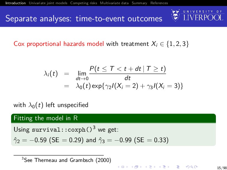
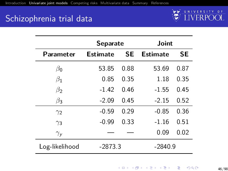
17. Introduction Univariate joint models Competing risks Multivariate data Summary References Separate analyses: time-to-event outcomes Cox proportional hazards model with treatment Xi ∈ {1, 2, 3} λi (t) = lim dt→0 P(t ≤ T < t + dt | T ≥ t) dt = λ0(t) exp{γ2I(Xi = 2) + γ3I(Xi = 3)} with λ0(t) left unspecified Fitting the model in R Using survival::coxph()3 we get: ˆ γ2 = −0.59 (SE = 0.29) and ˆ γ3 = −0.99 (SE = 0.33) 3See Therneau and Grambsch (2000) 15/98
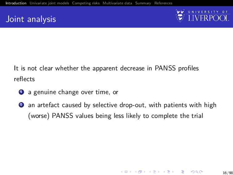
18. Introduction Univariate joint models Competing risks Multivariate data Summary References Joint analysis It is not clear whether the apparent decrease in PANSS profiles reflects 1 a genuine change over time, or 2 an artefact caused by selective drop-out, with patients with high (worse) PANSS values being less likely to complete the trial 16/98
19. Introduction Univariate joint models Competing risks Multivariate data Summary References Joint analysis In general, the primary focus for inference may be on: 1 Improving inference for a repeated measurement outcome subject to an informative dropout mechanism that is not of direct interest 2 Improving inference for a time-to-event outcome, whilst taking account of an intermittently and error-prone measured endogenous time-dependent variable 3 Studying the relationship between the two correlated processes In the previous slide, our focus was of type 1 17/98
20. Introduction Univariate joint models Competing risks Multivariate data Summary References Joint analysis Interest might also be about 1 Prediction4: given the measurement data for a patient up to time t, what is their survivorship distribution at time s > t? 2 Surrogacy5: when the clinical event is rare or takes a long time to reach, we want to use more easily measured markers as a substitute, which can usually lead to substantial sample size reduction and shorter trial duration. In other words, is [T | X, Y ] = [T|Y ]? 4e.g. Andrinopoulou et al. (2015) 5e.g. Xu and Zeger (2001) 18/98
21. Introduction Univariate joint models Competing risks Multivariate data Summary References Joint analysis What methods can we use to answer these sorts of questions? Separate analyses: simply ignore the association Naive models: Cox regression with time-varying covariate(s) assuming last-value carried forward Two-stage models: the LMM is first fitted separately, and the best linear unbiased predictors (BLUPS) of the random effects extracted and included in a time-varying covariate survival model Pattern mixture or selection models: factorize the joint distribution as either [Y , T] = [T] × [Y | T] = [Y ] × [T | Y ] Landmarking: refitting the survival model at sequential follow-up times conditional on subjects still in the risk set Joint models: focus of today’s workshop 19/98
22. Introduction Univariate joint models Competing risks Multivariate data Summary References Software implementations in R Advanced statistical methods have limited use if not readily and publicly available in software R is a free software environment for statistical computing and graphics It compiles and runs on a wide variety of UNIX platforms, Windows, and macOS 20/98
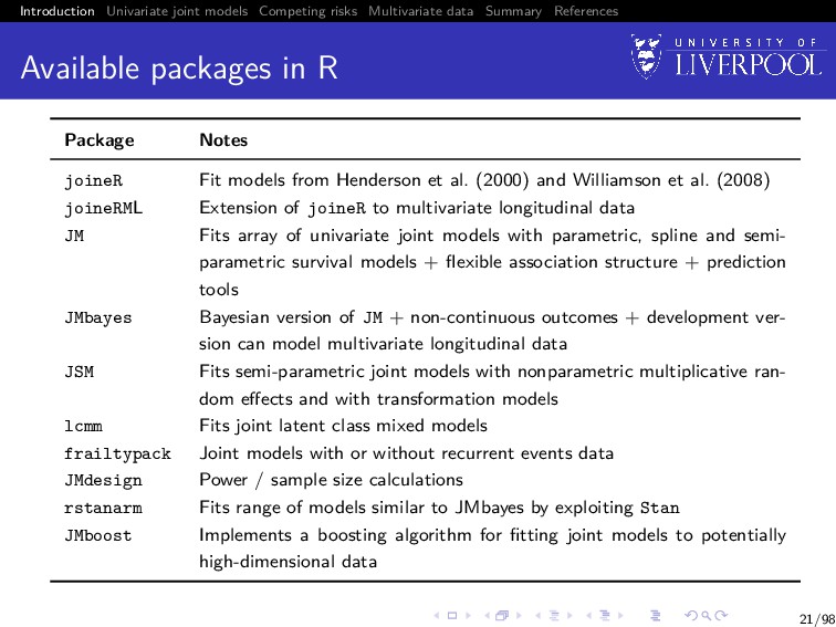
23. Introduction Univariate joint models Competing risks Multivariate data Summary References Available packages in R Package Notes joineR Fit models from Henderson et al. (2000) and Williamson et al. (2008) joineRML Extension of joineR to multivariate longitudinal data JM Fits array of univariate joint models with parametric, spline and semi- parametric survival models + flexible association structure + prediction tools JMbayes Bayesian version of JM + non-continuous outcomes + development ver- sion can model multivariate longitudinal data JSM Fits semi-parametric joint models with nonparametric multiplicative ran- dom effects and with transformation models lcmm Fits joint latent class mixed models frailtypack Joint models with or without recurrent events data JMdesign Power / sample size calculations rstanarm Fits range of models similar to JMbayes by exploiting Stan JMboost Implements a boosting algorithm for fitting joint models to potentially high-dimensional data 21/98
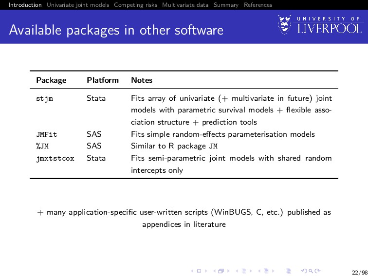
24. Introduction Univariate joint models Competing risks Multivariate data Summary References Available packages in other software Package Platform Notes stjm Stata Fits array of univariate (+ multivariate in future) joint models with parametric survival models + flexible asso- ciation structure + prediction tools JMFit SAS Fits simple random-effects parameterisation models %JM SAS Similar to R package JM jmxtstcox Stata Fits semi-parametric joint models with shared random intercepts only + many application-specific user-written scripts (WinBUGS, C, etc.) published as appendices in literature 22/98
25. Introduction Univariate joint models Competing risks Multivariate data Summary References Learning objectives 1 Recognise what problems joint models can be used for 2 Understand how joint models can be fitted (in frequentist framework) 3 Fit joint models in R independently 4 Interpret joint models for inference Everything discussed today stems from our own research and actual clinical questions using real clinical data 23/98
26. Introduction Univariate joint models Competing risks Multivariate data Summary References Univariate joint models 24/98
27. Introduction Univariate joint models Competing risks Multivariate data Summary References A brief history Originally motivated by AIDS research in which a biomarker such as CD4 lymphocyte count is determined intermittently and its relationship with time to seroconversion or death is of interest Seminal articles by Wulfsohn and Tsiatis (1997) and Henderson et al. (2000) contributed to a rapidly growing research field As of 2015: > 200 methodological papers and > 60 clinical applications of joint models 25/98
28. Introduction Univariate joint models Competing risks Multivariate data Summary References Conceptual principle Covariate data Longitudinal outcomes data Random effects 26/98
29. Introduction Univariate joint models Competing risks Multivariate data Summary References Conceptual principle Covariate data Time-to-event outcomes data Frailties 26/98
30. Introduction Univariate joint models Competing risks Multivariate data Summary References Conceptual principle Covariate data Time-to-event outcomes data Frailties Longitudinal outcomes data Random effects 26/98
31. Introduction Univariate joint models Competing risks Multivariate data Summary References Conceptual principle Covariate data Time-to-event outcomes data Frailties Longitudinal outcomes data Random effects 26/98
32. Introduction Univariate joint models Competing risks Multivariate data Summary References Data For each subject i = 1, . . . , n, we observe An ni -vector of observed longitudinal measurements for the longitudinal outcome: yi = (yi1, . . . , yini ) Observation times tij for j = 1, . . . , ni , which can differ between subjects (Ti , δi ), where Ti = min(T∗ i , Ci ), where T∗ i is the true event time, Ci corresponds to a potential right-censoring time, and δi is the failure indicator equal to 1 if the failure is observed (T∗ i ≤ Ci ) and 0 otherwise 27/98
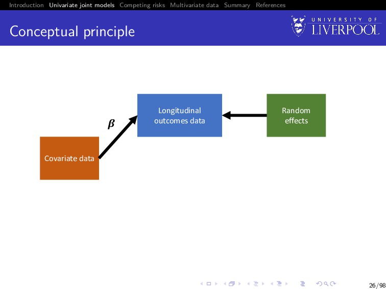
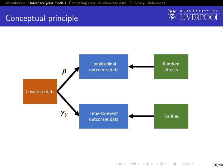
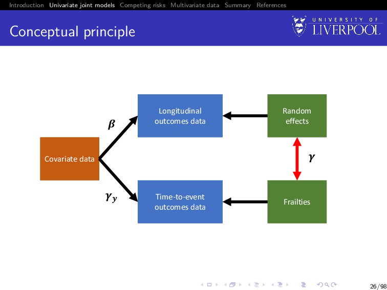
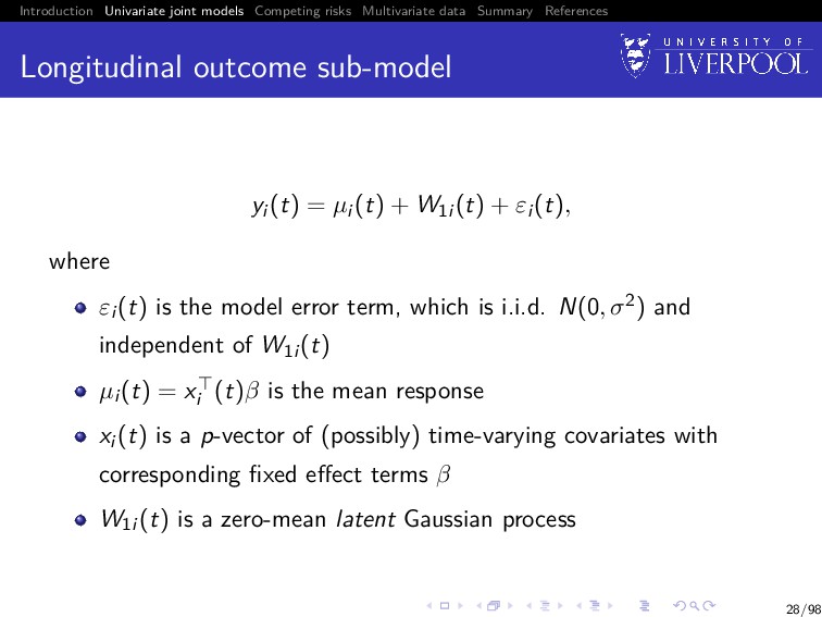
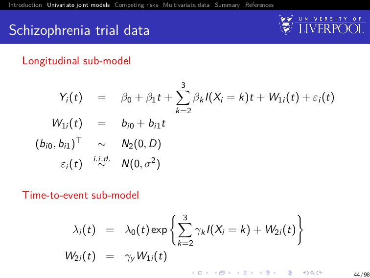
33. Introduction Univariate joint models Competing risks Multivariate data Summary References Longitudinal outcome sub-model yi (t) = µi (t) + W1i (t) + εi (t), where εi (t) is the model error term, which is i.i.d. N(0, σ2) and independent of W1i (t) µi (t) = xi (t)β is the mean response xi (t) is a p-vector of (possibly) time-varying covariates with corresponding fixed effect terms β W1i (t) is a zero-mean latent Gaussian process 28/98
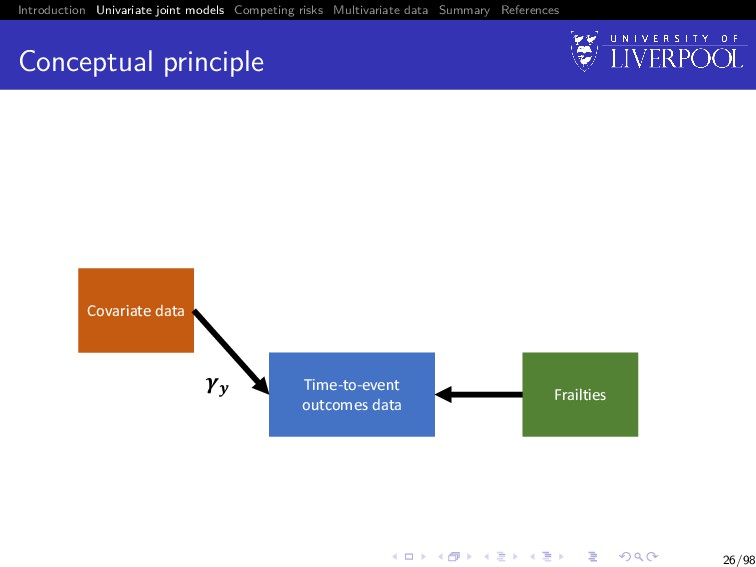
34. Introduction Univariate joint models Competing risks Multivariate data Summary References Time to event outcome sub-model λi (t) = λ0(t) exp vi (t)γv + W2i (t) , where λ0(·) is an unspecified baseline hazard function vi (t) is a q-vector of (possibly) time-varying covariates with corresponding fixed effect terms γv W2i (t) is a zero-mean latent Gaussian process, independent of the censoring process 29/98
35. Introduction Univariate joint models Competing risks Multivariate data Summary References Association structure W1(t) Following Laird and Ware (1982): W1i (t) = zi (t)bi , with bi ∼ N(0, D) 30/98
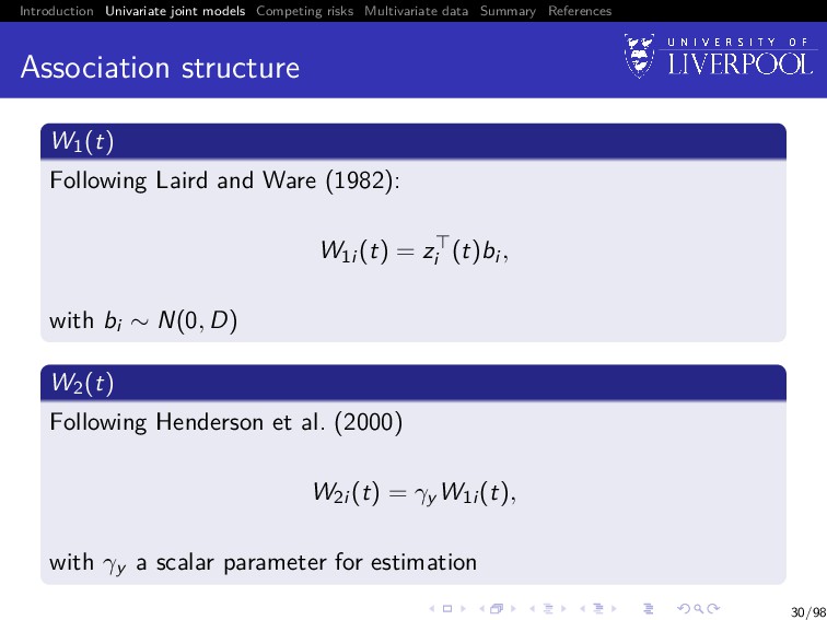
36. Introduction Univariate joint models Competing risks Multivariate data Summary References Association structure W1(t) Following Laird and Ware (1982): W1i (t) = zi (t)bi , with bi ∼ N(0, D) W2(t) Following Henderson et al. (2000) W2i (t) = γy W1i (t), with γy a scalar parameter for estimation 30/98
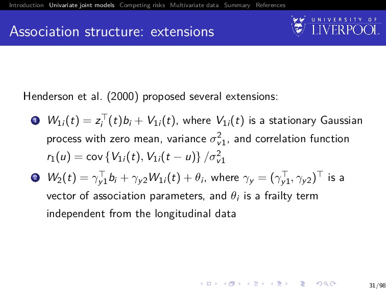
37. Introduction Univariate joint models Competing risks Multivariate data Summary References Association structure: extensions Henderson et al. (2000) proposed several extensions: 1 W1i (t) = zi (t)bi + V1i (t), where V1i (t) is a stationary Gaussian process with zero mean, variance σ2 v1 , and correlation function r1(u) = cov {V1i (t), V1i (t − u)} /σ2 v1 2 W2(t) = γy1 bi + γy2W1i (t) + θi , where γy = (γy1 , γy2) is a vector of association parameters, and θi is a frailty term independent from the longitudinal data 31/98
38. Introduction Univariate joint models Competing risks Multivariate data Summary References Association structure: alternatives Many other proposals for association structures in the literature: Current value parameterisation: W2i (t) = γy {µi (t) + W1i (t)} Random effects parameterisation: W2i (t) = γy1 bi Bivariate distribution: (W1i , W2i ) ∼ N(0, Ω) Random-slopes parameterisation: W2i (t) = γy1 {µi (t) + W1i (t)} + γy2 ∂ ∂t {µi (t) + W1i (t)} . . . 32/98
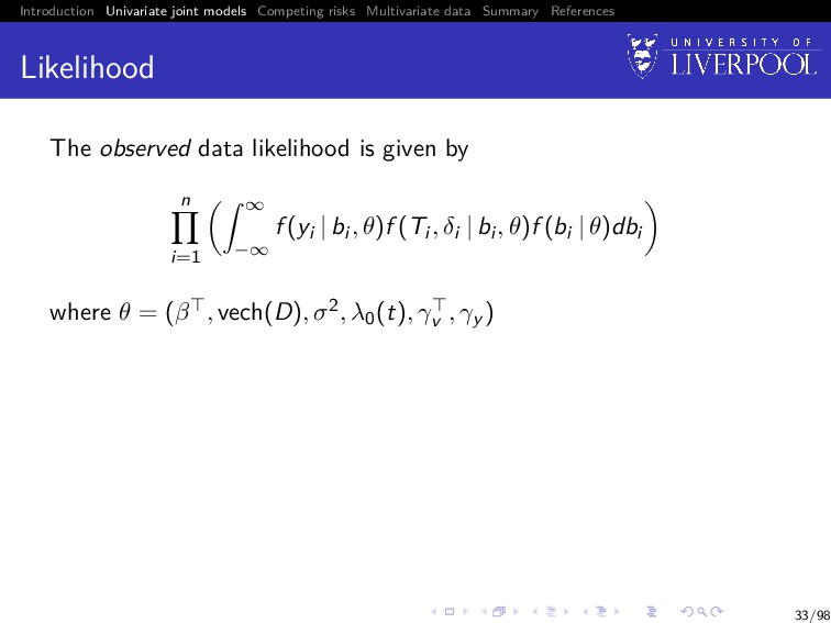
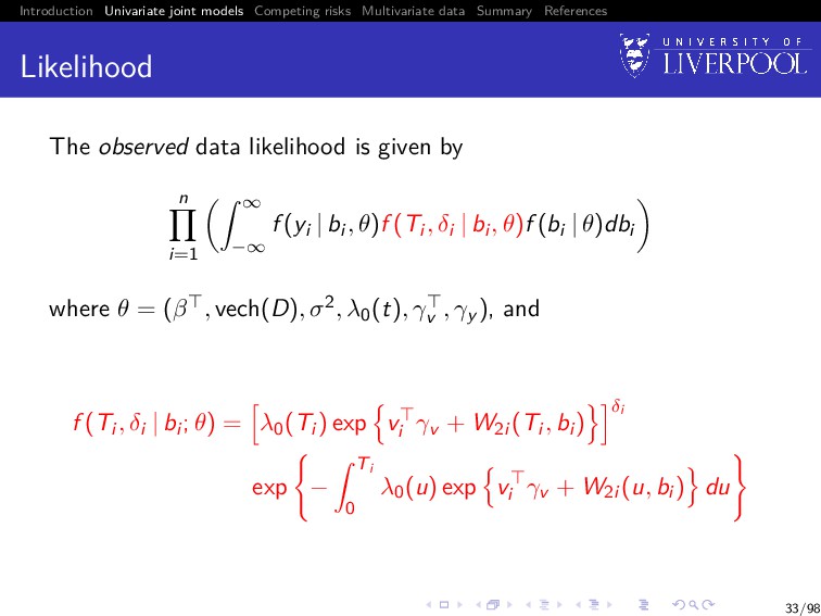
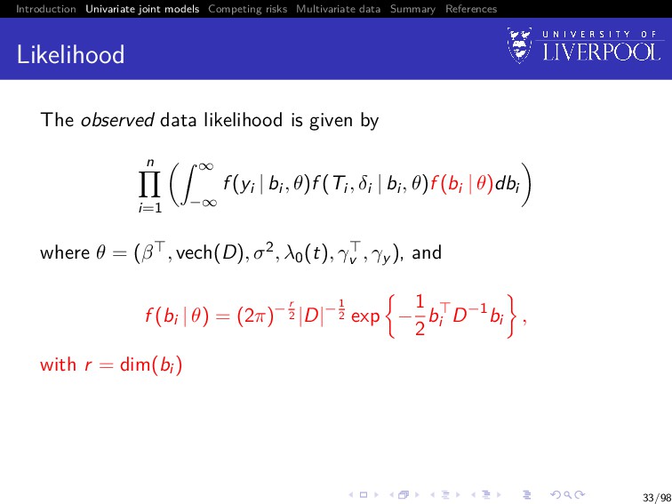
39. Introduction Univariate joint models Competing risks Multivariate data Summary References Likelihood The observed data likelihood is given by n i=1 ∞ −∞ f (yi | bi , θ)f (Ti , δi | bi , θ)f (bi | θ)dbi where θ = (β , vech(D), σ2, λ0(t), γv , γy ) 33/98
40. Introduction Univariate joint models Competing risks Multivariate data Summary References Likelihood The observed data likelihood is given by n i=1 ∞ −∞ f (yi | bi , θ)f (Ti , δi | bi , θ)f (bi | θ)dbi where θ = (β , vech(D), σ2, λ0(t), γv , γy ), and f (yi | bi , θ) = (2π)−ni 2 σ−ni exp − 1 2σ2 (yi − Xi β − Zi bi ) (yi − Xi β − Zi bi ) 33/98
41. Introduction Univariate joint models Competing risks Multivariate data Summary References Likelihood The observed data likelihood is given by n i=1 ∞ −∞ f (yi | bi , θ)f (Ti , δi | bi , θ)f (bi | θ)dbi where θ = (β , vech(D), σ2, λ0(t), γv , γy ), and f (Ti , δi | bi ; θ) = λ0(Ti ) exp vi γv + W2i (Ti , bi ) δi exp − Ti 0 λ0(u) exp vi γv + W2i (u, bi ) du 33/98
42. Introduction Univariate joint models Competing risks Multivariate data Summary References Likelihood The observed data likelihood is given by n i=1 ∞ −∞ f (yi | bi , θ)f (Ti , δi | bi , θ)f (bi | θ)dbi where θ = (β , vech(D), σ2, λ0(t), γv , γy ), and f (bi | θ) = (2π)− r 2 |D|−1 2 exp − 1 2 bi D−1bi , with r = dim(bi ) 33/98
43. Introduction Univariate joint models Competing risks Multivariate data Summary References Estimation Multiple approaches have been considered over the years: Markov chain Monte Carlo (MCMC) Direct likelihood maximisation (e.g. Newton-methods) Generalised estimating equations EM algorithm (treating the random effects as missing data) . . . 34/98
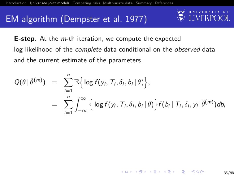
44. Introduction Univariate joint models Competing risks Multivariate data Summary References EM algorithm (Dempster et al. 1977) E-step. At the m-th iteration, we compute the expected log-likelihood of the complete data conditional on the observed data and the current estimate of the parameters. Q(θ | ˆ θ(m)) = n i=1 E log f (yi , Ti , δi , bi | θ) , = n i=1 ∞ −∞ log f (yi , Ti , δi , bi | θ) f (bi | Ti , δi , yi ; ˆ θ(m))dbi 35/98
45. Introduction Univariate joint models Competing risks Multivariate data Summary References EM algorithm (Dempster et al. 1977) E-step. At the m-th iteration, we compute the expected log-likelihood of the complete data conditional on the observed data and the current estimate of the parameters. Q(θ | ˆ θ(m)) = n i=1 E log f (yi , Ti , δi , bi | θ) , = n i=1 ∞ −∞ log f (yi , Ti , δi , bi | θ) f (bi | Ti , δi , yi ; ˆ θ(m))dbi M-step. We maximise Q(θ | ˆ θ(m)) with respect to θ. namely, ˆ θ(m+1) = arg max θ Q(θ | ˆ θ(m)) 35/98
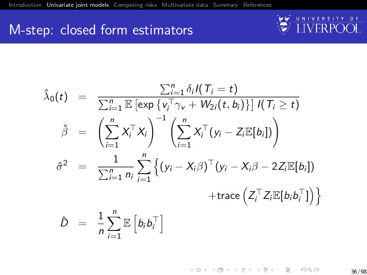
46. Introduction Univariate joint models Competing risks Multivariate data Summary References M-step: closed form estimators ˆ λ0(t) = n i=1 δi I(Ti = t) n i=1 E exp vi γv + W2i (t, bi ) I(Ti ≥ t) ˆ β = n i=1 Xi Xi −1 n i=1 Xi (yi − Zi E[bi ]) ˆ σ2 = 1 n i=1 ni n i=1 (yi − Xi β) (yi − Xi β − 2Zi E[bi ]) +trace Zi Zi E[bi bi ] ˆ D = 1 n n i=1 E bi bi 36/98
47. Introduction Univariate joint models Competing risks Multivariate data Summary References M-step: non-closed form estimators There is no closed form update for γ = (γv , γy ) , so use a one-step Newton-Raphson iteration ˆ γ(m+1) = ˆ γ(m) + I ˆ γ(m) −1 S ˆ γ(m) , where S(γ) = n i=1 δi E [˜ vi (Ti )] − Ti 0 λ0(u)E ˜ vi (u) exp{˜ vi (u)γ} du I(γ) = − ∂ ∂γ S(γ) with ˜ vi (t) = vi , zi (t)bi a (q + 1)–vector6 6Generalises to a (q + |γy |)–vector if γy is a vector 37/98
48. Introduction Univariate joint models Competing risks Multivariate data Summary References E-step Need to calculate several multi-dimensional expectations of the form E [h(bi )] = · · · ∞ −∞ h(bi )f (bi | Ti , δi , yi , ˆ θ)dbi 38/98
49. Introduction Univariate joint models Competing risks Multivariate data Summary References E-step Need to calculate several multi-dimensional expectations of the form E [h(bi )] = · · · ∞ −∞ h(bi )f (bi | Ti , δi , yi , ˆ θ)dbi 38/98
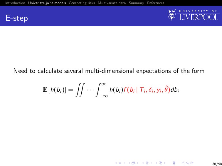
50. Introduction Univariate joint models Competing risks Multivariate data Summary References E-step E h(bi ) | Ti , δi , yi ; ˆ θ = ∞ −∞ h(bi )f (bi | yi ; ˆ θ)f (Ti , δi | bi ; ˆ θ)dbi ∞ −∞ f (bi | yi ; ˆ θ)f (Ti , δi | bi ; ˆ θ)dbi , where h(·) = any known fuction, bi | yi , θ ∼ N Ai σ−2Zi (yi − Xi β) , Ai , and Ai = σ−2Zi Zi + D−1 −1 39/98
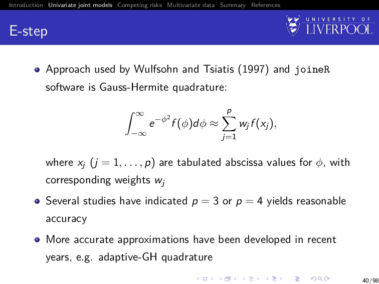
51. Introduction Univariate joint models Competing risks Multivariate data Summary References E-step Approach used by Wulfsohn and Tsiatis (1997) and joineR software is Gauss-Hermite quadrature: ∞ −∞ e−φ2 f (φ)dφ ≈ p j=1 wjf (xj), where xj (j = 1, . . . , p) are tabulated abscissa values for φ, with corresponding weights wj Several studies have indicated p = 3 or p = 4 yields reasonable accuracy More accurate approximations have been developed in recent years, e.g. adaptive-GH quadrature 40/98
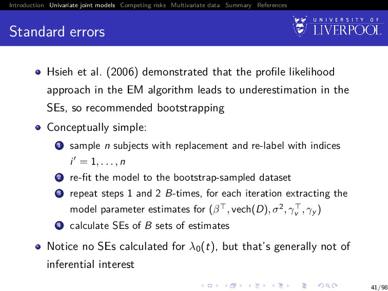
52. Introduction Univariate joint models Competing risks Multivariate data Summary References Standard errors Hsieh et al. (2006) demonstrated that the profile likelihood approach in the EM algorithm leads to underestimation in the SEs, so recommended bootstrapping Conceptually simple: 1 sample n subjects with replacement and re-label with indices i = 1, . . . , n 2 re-fit the model to the bootstrap-sampled dataset 3 repeat steps 1 and 2 B-times, for each iteration extracting the model parameter estimates for (β , vech(D), σ2, γv , γy ) 4 calculate SEs of B sets of estimates Notice no SEs calculated for λ0(t), but that’s generally not of inferential interest 41/98
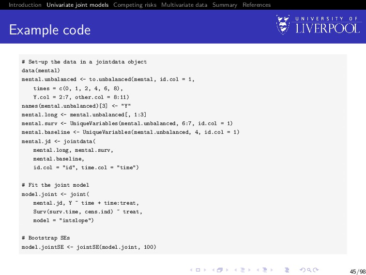
53. Introduction Univariate joint models Competing risks Multivariate data Summary References Software We can implement all of this in the R package joineR, with the general recipe: 1 Create a jointdata object using the joineR::jointdata() function 2 Fit a joint model using the joineR::joint() function 3 Calculate SEs using joineR::jointSE() function Each piece can be used in separate auxiliary functions along the way 42/98
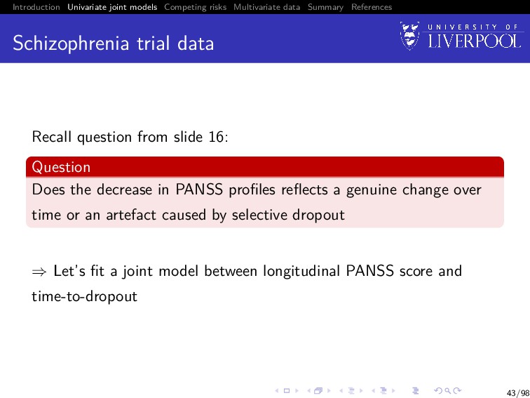
54. Introduction Univariate joint models Competing risks Multivariate data Summary References Schizophrenia trial data Recall question from slide 16: Question Does the decrease in PANSS profiles reflects a genuine change over time or an artefact caused by selective dropout ⇒ Let’s fit a joint model between longitudinal PANSS score and time-to-dropout 43/98
55. Introduction Univariate joint models Competing risks Multivariate data Summary References Schizophrenia trial data Longitudinal sub-model Yi (t) = β0 + β1t + 3 k=2 βkI(Xi = k)t + W1i (t) + εi (t) W1i (t) = bi0 + bi1t (bi0, bi1) ∼ N2(0, D) εi (t) i.i.d. ∼ N(0, σ2) Time-to-event sub-model λi (t) = λ0(t) exp 3 k=2 γkI(Xi = k) + W2i (t) W2i (t) = γy W1i (t) 44/98
56. Introduction Univariate joint models Competing risks Multivariate data Summary References Example code # Set-up the data in a jointdata object data(mental) mental.unbalanced <- to.unbalanced(mental, id.col = 1, times = c(0, 1, 2, 4, 6, 8), Y.col = 2:7, other.col = 8:11) names(mental.unbalanced)[3] <- "Y" mental.long <- mental.unbalanced[, 1:3] mental.surv <- UniqueVariables(mental.unbalanced, 6:7, id.col = 1) mental.baseline <- UniqueVariables(mental.unbalanced, 4, id.col = 1) mental.jd <- jointdata( mental.long, mental.surv, mental.baseline, id.col = "id", time.col = "time") # Fit the joint model model.joint <- joint( mental.jd, Y ˜ time + time:treat, Surv(surv.time, cens.ind) ˜ treat, model = "intslope") # Bootstrap SEs model.jointSE <- jointSE(model.joint, 100) 45/98
57. Introduction Univariate joint models Competing risks Multivariate data Summary References Schizophrenia trial data Separate Joint Parameter Estimate SE Estimate SE β0 53.85 0.88 53.69 0.87 β1 0.85 0.35 1.18 0.35 β2 -1.42 0.46 -1.55 0.45 β3 -2.09 0.45 -2.15 0.52 γ2 -0.59 0.29 -0.85 0.36 γ3 -0.99 0.33 -1.16 0.51 γy — — 0.09 0.02 Log-likelihood -2873.3 -2840.9 46/98
58. Introduction Univariate joint models Competing risks Multivariate data Summary References Extension I: Competing risks events 47/98
59. Introduction Univariate joint models Competing risks Multivariate data Summary References Motivation Joint models generally consider survival data that allows for one event with a single mode of failure and an assumption of independent censoring When there are several reasons why the failure event can occur, or some informative censoring occurs, it is known as competing risks 48/98
60. Introduction Univariate joint models Competing risks Multivariate data Summary References SANAD trial data SANAD (Standard And New Antiepileptic Drugs) was a non-blinded randomized control trial recruiting patients with epilepsy to test anti-epilepsy drugs (AEDs) Patients were randomized to one of 5 antiepilepsy drugs (AEDs) Subgroup analysis (n = 605 patients) comparing 2 drugs: LTG (newer drug) vs. CBZ (standard) 49/98
61. Introduction Univariate joint models Competing risks Multivariate data Summary References SANAD trial data Primary outcome was time to treatment failure, defined as the time to withdrawal of a randomised drug or addition of another/switch to an alternative AED Patients decided to switch to an alternative AED because of Inadequate seizure control (ISC; n = 94, 15%) Unacceptable adverse effects (UAE; n = 120, 20%) 50/98
62. Introduction Univariate joint models Competing risks Multivariate data Summary References Clinical question Question Is LTG superior to CBZ in terms of (a) seizure control and (b) tolerability? 51/98
63. Introduction Univariate joint models Competing risks Multivariate data Summary References Rationale for competing events Should we just analyse composite time-to-treatment failure for any reason? 52/98
64. Introduction Univariate joint models Competing risks Multivariate data Summary References Rationale for competing events Should we just analyse composite time-to-treatment failure for any reason? No: assumes reasons of failure are of equal importance (which may not be the case): Loss of driving license due to continued seizures Side effects such as nausea, dizziness or rash 52/98
65. Introduction Univariate joint models Competing risks Multivariate data Summary References Original results LTG is significantly more toler- able than CBZ 0.0 0.2 0.4 0.6 0.8 1.0 UAE Years Probability CBZ LTG 0 1 2 3 4 5 6 53/98
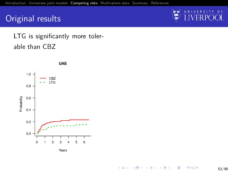
66. Introduction Univariate joint models Competing risks Multivariate data Summary References Original results LTG is significantly more toler- able than CBZ 0.0 0.2 0.4 0.6 0.8 1.0 UAE Years Probability CBZ LTG 0 1 2 3 4 5 6 LTG is similar to CBZ in terms of seizure control 0.0 0.2 0.4 0.6 0.8 1.0 ISC Years Probability CBZ LTG 0 1 2 3 4 5 6 53/98
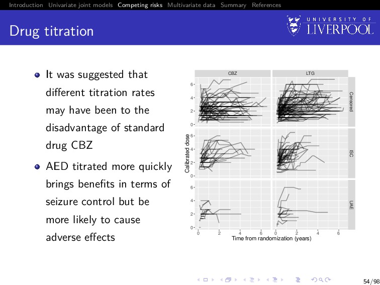
67. Introduction Univariate joint models Competing risks Multivariate data Summary References Drug titration It was suggested that different titration rates may have been to the disadvantage of standard drug CBZ AED titrated more quickly brings benefits in terms of seizure control but be more likely to cause adverse effects CBZ LTG 0 2 4 6 0 2 4 6 0 2 4 6 Censored ISC UAE 0 2 4 6 0 2 4 6 Time from randomization (years) Calibrated dose 54/98
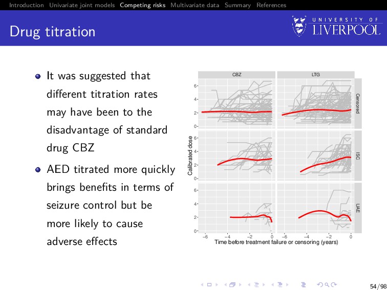
68. Introduction Univariate joint models Competing risks Multivariate data Summary References Drug titration It was suggested that different titration rates may have been to the disadvantage of standard drug CBZ AED titrated more quickly brings benefits in terms of seizure control but be more likely to cause adverse effects CBZ LTG Censored ISC UAE −6 −4 −2 0 −6 −4 −2 0 0 2 4 6 0 2 4 6 0 2 4 6 Time before treatment failure or censoring (years) Calibrated dose 54/98
69. Introduction Univariate joint models Competing risks Multivariate data Summary References Revised clinical questions Questions 1 Is drug titration associated with time to treatment failure for each cause? 2 After adjusting for drug titration is LTG still superior to CBZ in terms of UAE and ISC? 55/98
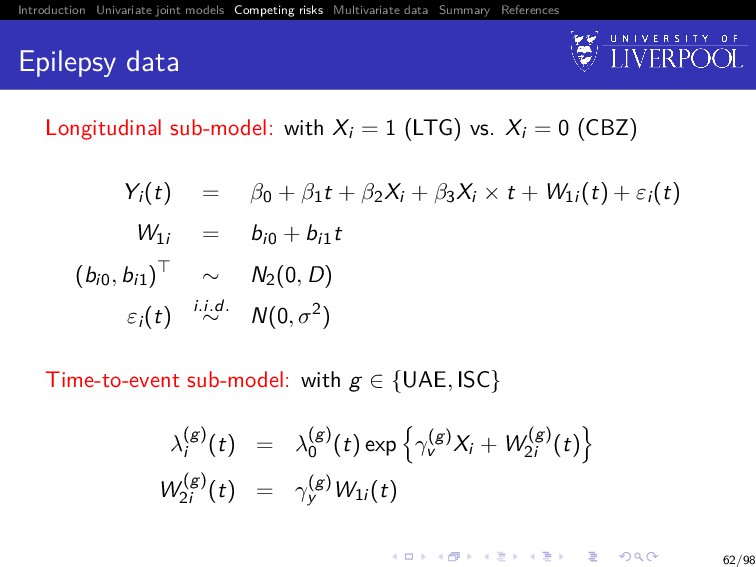
70. Introduction Univariate joint models Competing risks Multivariate data Summary References Data For each subject i = 1, . . . , n, we observe An ni -vector of observed longitudinal measurements for the longitudinal outcome: yi = (yi1, . . . , yini ) Observation times tij for j = 1, . . . , ni , which can differ between subjects (Ti , δi ), where Ti = min(T∗ i , Ci ), where T∗ i is the true event time, Ci corresponds to a potential non-informative right-censoring time, and δi is the failure indicator equal to g (g = 1, . . . , G) if the failure is observed (T∗ i ≤ Ci ) and due to cause g, and 0 otherwise 56/98
71. Introduction Univariate joint models Competing risks Multivariate data Summary References Model Longitudinal sub-model: same as for the univariate joint model Time-to-event sub-model: cause-specific hazards model 57/98
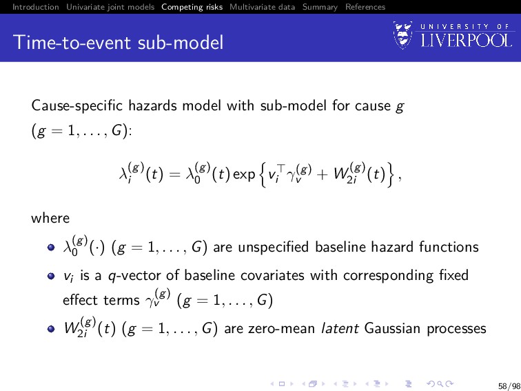
72. Introduction Univariate joint models Competing risks Multivariate data Summary References Time-to-event sub-model Cause-specific hazards model with sub-model for cause g (g = 1, . . . , G): λ(g) i (t) = λ(g) 0 (t) exp vi γ(g) v + W (g) 2i (t) , where λ(g) 0 (·) (g = 1, . . . , G) are unspecified baseline hazard functions vi is a q-vector of baseline covariates with corresponding fixed effect terms γ(g) v (g = 1, . . . , G) W (g) 2i (t) (g = 1, . . . , G) are zero-mean latent Gaussian processes 58/98
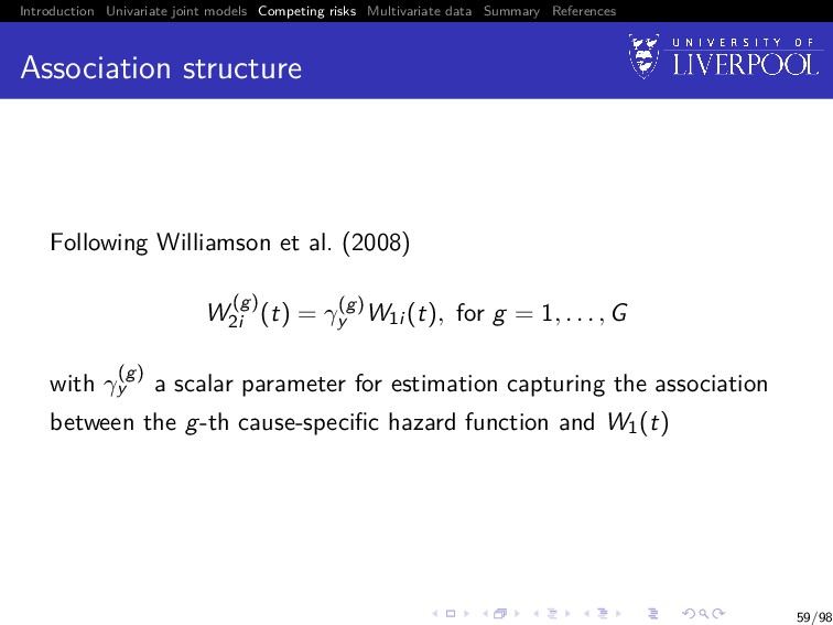
73. Introduction Univariate joint models Competing risks Multivariate data Summary References Association structure Following Williamson et al. (2008) W (g) 2i (t) = γ(g) y W1i (t), for g = 1, . . . , G with γ(g) y a scalar parameter for estimation capturing the association between the g-th cause-specific hazard function and W1(t) 59/98
74. Introduction Univariate joint models Competing risks Multivariate data Summary References Estimation & standard errors EM algorithm as per before, with exception that we now estimate G-pairs of λ(g) 0 (t), γ(g) y during the M-step Standard errors estimated using same bootstrap method 60/98
75. Introduction Univariate joint models Competing risks Multivariate data Summary References Software We can fit these models in joineR using the same general work-flow as for the single failure type joint model joineR::joint() automatically detects presence of competing risks7 Currently limited to 2 failure types 7Requires failure types to be coded as 0 (censored), 1 (first failure type), 2 (second failure type). 61/98
76. Introduction Univariate joint models Competing risks Multivariate data Summary References Epilepsy data Longitudinal sub-model: with Xi = 1 (LTG) vs. Xi = 0 (CBZ) Yi (t) = β0 + β1t + β2Xi + β3Xi × t + W1i (t) + εi (t) W1i = bi0 + bi1t (bi0, bi1) ∼ N2(0, D) εi (t) i.i.d. ∼ N(0, σ2) Time-to-event sub-model: with g ∈ {UAE, ISC} λ(g) i (t) = λ(g) 0 (t) exp γ(g) v Xi + W (g) 2i (t) W (g) 2i (t) = γ(g) y W1i (t) 62/98
77. Introduction Univariate joint models Competing risks Multivariate data Summary References Example code # Setup joint data data(epileptic) epileptic$interaction <- with(epileptic, time * (treat == "LTG")) longitudinal <- epileptic[, c(1:3, 13)] survival <- UniqueVariables(epileptic, c(4, 6), "id") baseline <- UniqueVariables(epileptic, "treat", "id") data <- jointdata(longitudinal = longitudinal, survival = survival, baseline = baseline, id.col = "id", time.col = "time") # Fit joint model fit2 <- joint(data = data, long.formula = dose ˜ time + treat + interaction, surv.formula = Surv(with.time, with.status2) ˜ treat, longsep = FALSE, survsep = FALSE) 63/98
78. Introduction Univariate joint models Competing risks Multivariate data Summary References Epilepsy data Est. SE 95% CI β0 (Intercept) 1.9730 0.0512 (1.8701, 2.0803) β1 time 0.0004 0.0001 (0.0002, 0.0005) β2 LTG -0.1381 0.0720 (-0.2908, -0.0307) β3 time × LTG 0.0006 0.0001 (0.0003, 0.0009) γ(UAE) v LTG -0.6602 0.2008 (-1.1063, -0.2338) γ(UAE) y Titration -0.9259 0.2600 (-1.4707, -0.4510) γ(ISC) v LTG 0.0272 0.1811 (-0.3940, 0.3306) γ(ISC) y Titration 0.5894 0.0873 (0.4031, 0.7513) 64/98
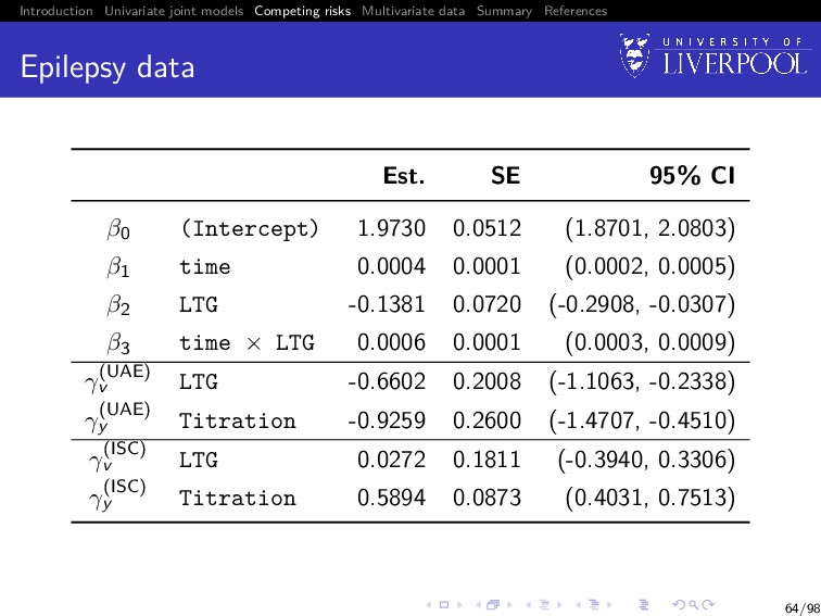
79. Introduction Univariate joint models Competing risks Multivariate data Summary References Conclusion Is LTG superior to CBZ after adjusting for titration in terms of UAE? ISC? If LTG is titrated at the same rate as CBZ, the beneficial effect of LTG on UAE would still be evident LTG and CBZ still appear to provide similar seizure control 65/98
80. Introduction Univariate joint models Competing risks Multivariate data Summary References Extension II: Multiple longitudinal outcomes 66/98
81. Introduction Univariate joint models Competing risks Multivariate data Summary References Motivation Clinical studies often repeatedly measure multiple biomarkers or other measurements and an event time Research has predominantly focused on single measurement outcomes Harnessing all available information in a single model is advantageous and should lead to improved estimation and predictions 67/98
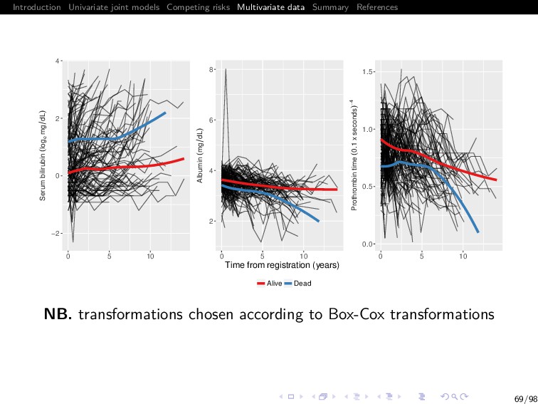
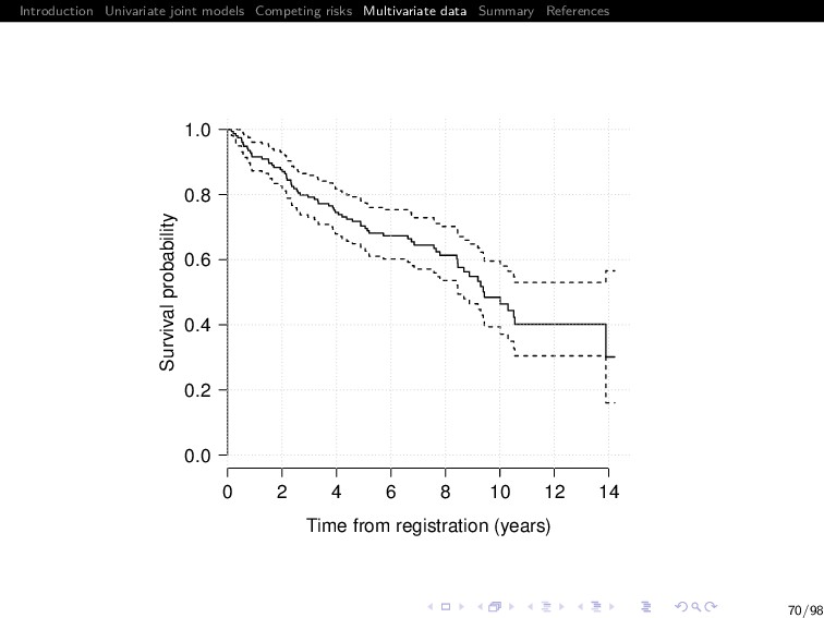
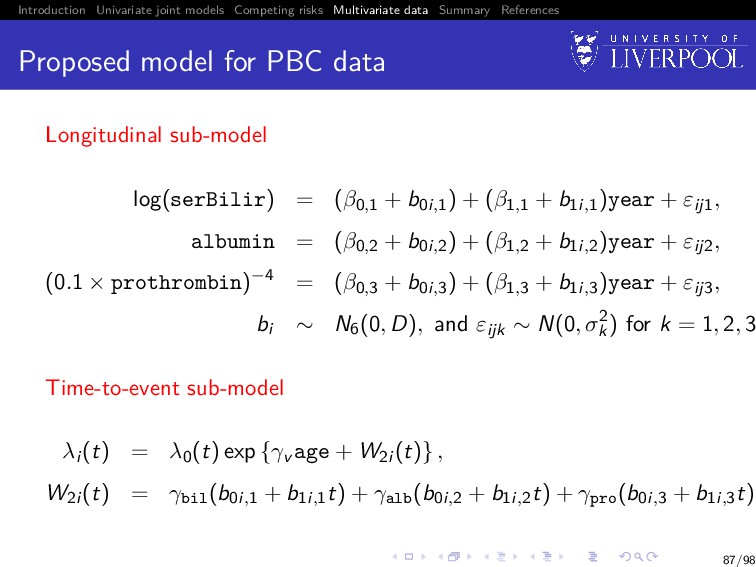
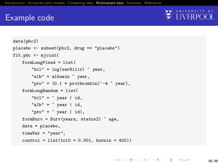
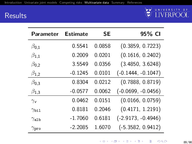
82. Introduction Univariate joint models Competing risks Multivariate data Summary References The Mayo Clinic PBC data Primary biliary cirrhosis (PBC) is a chronic liver disease characterized by inflammatory destruction of the small bile ducts, which eventually leads to cirrhosis of the liver (Murtaugh et al. 1994) We analyse a subset of 154 patients randomized to placebo Multiple biomarkers repeatedly measured at intermittent times: 1 serum bilirubin (mg/dl) 2 serum albumin (mg/dl) 3 prothrombin time (seconds) Patients drop out if they die (ndie = 69, 44.8%) 68/98
83. Introduction Univariate joint models Competing risks Multivariate data Summary References Prothrombin time (0.1 x seconds)−4 Albumin (mg dL) Serum bilirubin (loge mg dL) 0 5 10 0 5 10 0 5 10 0.0 0.5 1.0 1.5 2 4 6 8 −2 0 2 4 Time from registration (years) Alive Dead NB. transformations chosen according to Box-Cox transformations 69/98
84. Introduction Univariate joint models Competing risks Multivariate data Summary References 0 2 4 6 8 10 12 14 0.0 0.2 0.4 0.6 0.8 1.0 Time from registration (years) Survival probability 70/98
85. Introduction Univariate joint models Competing risks Multivariate data Summary References What is the state of the field? A large number of models published over recent years incorporating different outcome types; distributions, multivariate event times; estimation approaches; association structures; disease areas; etc. Early adoption into clinical literature, but a lack of software! 71/98
86. Introduction Univariate joint models Competing risks Multivariate data Summary References Data For each subject i = 1, . . . , n, we observe yi = (yi1 , . . . , yiK ) is the K-variate continuous outcome vector, where each yik denotes an (nik × 1)-vector of observed longitudinal measurements for the k-th outcome type: yik = (yi1k, . . . , yinik k) Observation times tijk for j = 1, . . . , nik, which can differ between subjects and outcomes (Ti , δi ), where Ti = min(T∗ i , Ci ), where T∗ i is the true event time, Ci corresponds to a potential right-censoring time, and δi is the failure indicator equal to 1 if the failure is observed (T∗ i ≤ Ci ) and 0 otherwise 72/98
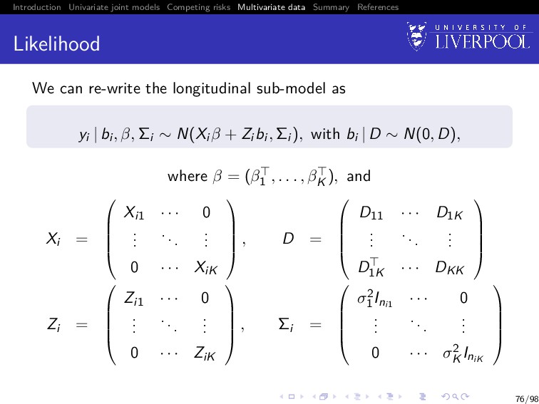
87. Introduction Univariate joint models Competing risks Multivariate data Summary References Longitudinal sub-model For the k-th outcome (k = 1, . . . , K) yik(t) = µik(t) + W (k) 1i (t) + εik(t), where εik(t) is the model error term, which is i.i.d. N(0, σ2 k ) and independent of W (k) 1i (t) µik(t) = xik (t)βk is the mean response xik(t) is a pk-vector of (possibly) time-varying covariates with corresponding fixed effect terms βk W (k) 1i (t) is a zero-mean latent Gaussian process 73/98
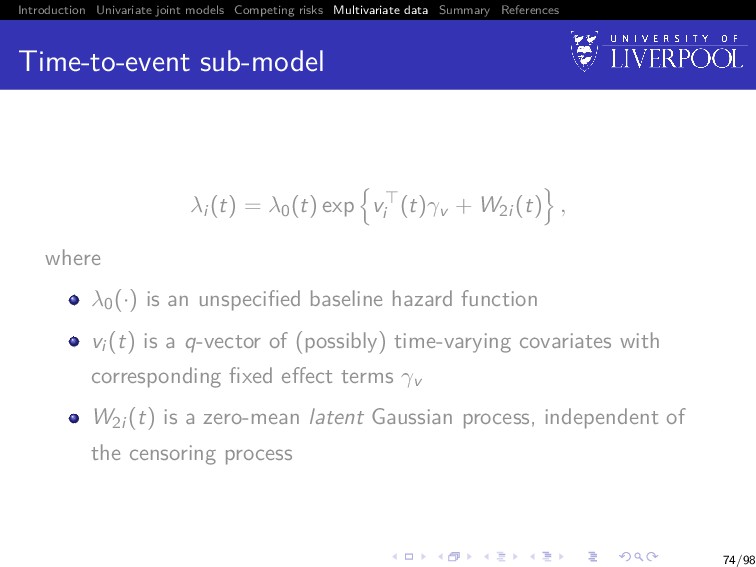
88. Introduction Univariate joint models Competing risks Multivariate data Summary References Time-to-event sub-model λi (t) = λ0(t) exp vi (t)γv + W2i (t) , where λ0(·) is an unspecified baseline hazard function vi (t) is a q-vector of (possibly) time-varying covariates with corresponding fixed effect terms γv W2i (t) is a zero-mean latent Gaussian process, independent of the censoring process 74/98
89. Introduction Univariate joint models Competing risks Multivariate data Summary References Association structure Extending Laird and Ware (1982) to the multivariate case: W (k) 1i (t) = zik (t)bik 75/98
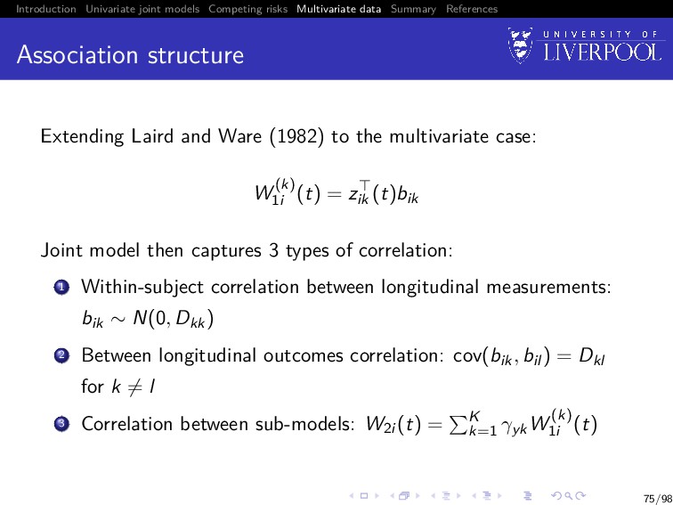
90. Introduction Univariate joint models Competing risks Multivariate data Summary References Association structure Extending Laird and Ware (1982) to the multivariate case: W (k) 1i (t) = zik (t)bik Joint model then captures 3 types of correlation: 1 Within-subject correlation between longitudinal measurements: bik ∼ N(0, Dkk) 2 Between longitudinal outcomes correlation: cov(bik, bil ) = Dkl for k = l 3 Correlation between sub-models: W2i (t) = K k=1 γykW (k) 1i (t) 75/98
91. Introduction Univariate joint models Competing risks Multivariate data Summary References Likelihood We can re-write the longitudinal sub-model as yi | bi , β, Σi ∼ N(Xi β + Zi bi , Σi ), with bi | D ∼ N(0, D), where β = (β1 , . . . , βK ), and Xi =      Xi1 · · · 0 . . . ... . . . 0 · · · XiK      , Zi =      Zi1 · · · 0 . . . ... . . . 0 · · · ZiK      , D =      D11 · · · D1K . . . ... . . . D1K · · · DKK      Σi =      σ2 1 Ini1 · · · 0 . . . ... . . . 0 · · · σ2 K IniK      76/98
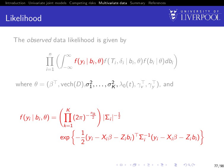
92. Introduction Univariate joint models Competing risks Multivariate data Summary References Likelihood The observed data likelihood is given by n i=1 ∞ −∞ f (yi | bi , θ)f (Ti , δi | bi , θ)f (bi | θ)dbi where θ = (β , vech(D),σ2 1 , . . . , σ2 K , λ0(t), γv , γy ) 77/98
93. Introduction Univariate joint models Competing risks Multivariate data Summary References Likelihood The observed data likelihood is given by n i=1 ∞ −∞ f (yi | bi , θ)f (Ti , δi | bi , θ)f (bi | θ)dbi where θ = (β , vech(D),σ2 1 , . . . , σ2 K , λ0(t), γv , γy ), and f (yi | bi , θ) = K k=1 (2π)−nik 2 |Σi |−1 2 exp − 1 2 (yi − Xi β − Zi bi ) Σ−1 i (yi − Xi β − Zi bi ) 77/98
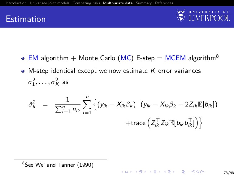
94. Introduction Univariate joint models Competing risks Multivariate data Summary References Estimation EM algorithm + Monte Carlo (MC) E-step = MCEM algorithm8 M-step identical except we now estimate K error variances σ2 1 , . . . , σ2 K as ˆ σ2 k = 1 n i=1 nik n i=1 (yik − Xikβk) (yik − Xikβk − 2ZikE[bik]) +trace Zik ZikE[bikbik ] 8See Wei and Tanner (1990) 78/98
95. Introduction Univariate joint models Competing risks Multivariate data Summary References E-step E h(bi ) | Ti , δi , yi ; ˆ θ = ∞ −∞ h(bi )f (bi | yi ; ˆ θ)f (Ti , δi | bi ; ˆ θ)dbi ∞ −∞ f (bi | yi ; ˆ θ)f (Ti , δi | bi ; ˆ θ)dbi , where h(·) = any known fuction, bi | yi , θ ∼ N Ai Zi Σ−1 i (yi − Xi β) , Ai , and Ai = Zi Σ−1 i Zi + D−1 −1 79/98
96. Introduction Univariate joint models Competing risks Multivariate data Summary References Monte Carlo E-step Replace the Gauss-Hermite quadrature with a Monte Carlo approximation for scalability with increasing K and/or dim(bi ) E h(bi ) | Ti , δi , yi ; ˆ θ = ∞ −∞ h(bi )f (bi | yi ; ˆ θ)f (Ti , δi | bi ; ˆ θ)dbi ∞ −∞ f (bi | yi ; ˆ θ)f (Ti , δi | bi ; ˆ θ)dbi , 80/98
97. Introduction Univariate joint models Competing risks Multivariate data Summary References Monte Carlo E-step Replace the Gauss-Hermite quadrature with a Monte Carlo approximation for scalability with increasing K and/or dim(bi ) E h(bi ) | Ti , δi , yi ; ˆ θ ≈ 1 N N d=1 h b(d) i f Ti , δi | b(d) i ; ˆ θ 1 N N d=1 f Ti , δi | b(d) i ; ˆ θ where b(1) i , b(2) i , . . . , b(N) i are a random sample from bi | yi , θ 80/98
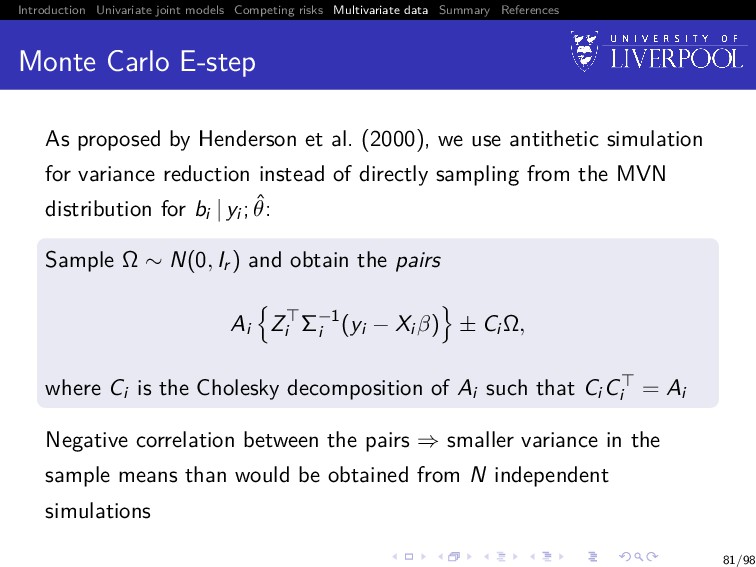
98. Introduction Univariate joint models Competing risks Multivariate data Summary References Monte Carlo E-step As proposed by Henderson et al. (2000), we use antithetic simulation for variance reduction instead of directly sampling from the MVN distribution for bi | yi ; ˆ θ: Sample Ω ∼ N(0, Ir ) and obtain the pairs Ai Zi Σ−1 i (yi − Xi β) ± Ci Ω, where Ci is the Cholesky decomposition of Ai such that Ci Ci = Ai Negative correlation between the pairs ⇒ smaller variance in the sample means than would be obtained from N independent simulations 81/98
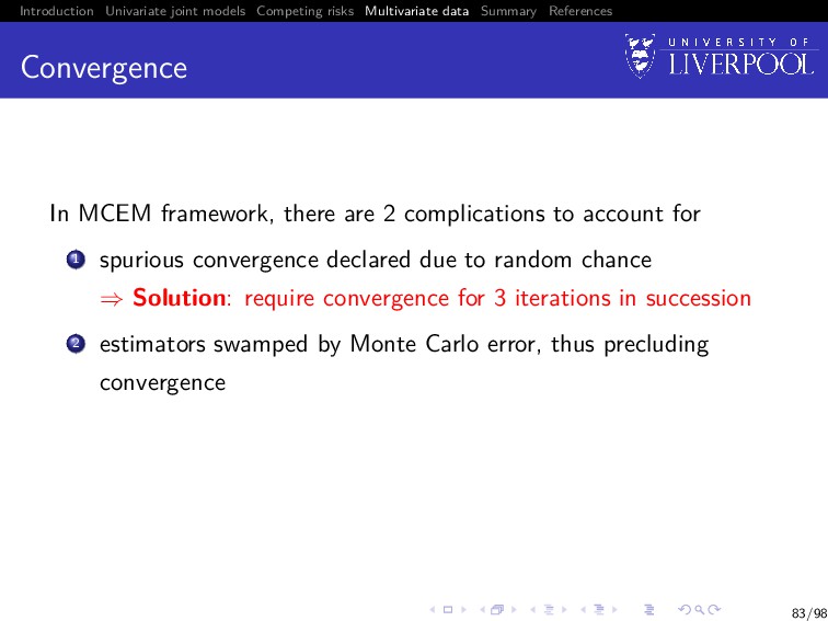
99. Introduction Univariate joint models Competing risks Multivariate data Summary References Convergence In standard EM, convergence usually declared at (m + 1)-th iteration if one of the following criteria satisfied 1 Relative change: ∆(m+1) rel = max |ˆ θ(m+1)−ˆ θ(m)| |ˆ θ(m)|+ 1 < 0 2 Absolute change: ∆(m+1) abs = max |ˆ θ(m+1) − ˆ θ(m)| < 2 for some choice of 0, 1, and 2 Note: joineR uses criterion #2 82/98
100. Introduction Univariate joint models Competing risks Multivariate data Summary References Convergence In MCEM framework, there are 2 complications to account for 83/98
101. Introduction Univariate joint models Competing risks Multivariate data Summary References Convergence In MCEM framework, there are 2 complications to account for 1 spurious convergence declared due to random chance 83/98
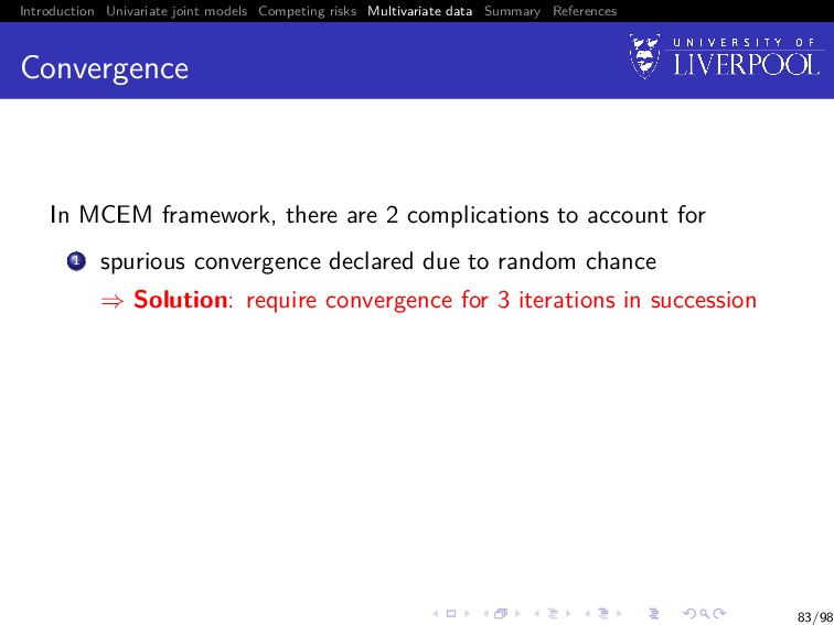
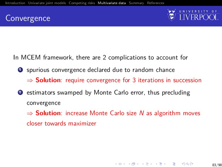
102. Introduction Univariate joint models Competing risks Multivariate data Summary References Convergence In MCEM framework, there are 2 complications to account for 1 spurious convergence declared due to random chance ⇒ Solution: require convergence for 3 iterations in succession 83/98
103. Introduction Univariate joint models Competing risks Multivariate data Summary References Convergence In MCEM framework, there are 2 complications to account for 1 spurious convergence declared due to random chance ⇒ Solution: require convergence for 3 iterations in succession 2 estimators swamped by Monte Carlo error, thus precluding convergence 83/98
104. Introduction Univariate joint models Competing risks Multivariate data Summary References Convergence In MCEM framework, there are 2 complications to account for 1 spurious convergence declared due to random chance ⇒ Solution: require convergence for 3 iterations in succession 2 estimators swamped by Monte Carlo error, thus precluding convergence ⇒ Solution: increase Monte Carlo size N as algorithm moves closer towards maximizer 83/98
105. Introduction Univariate joint models Competing risks Multivariate data Summary References Convergence Using large N when far from maximizer = computationally inefficient Using small N when close to maximizer = unlikely to detect convergence Solution (proposed by Ripatti et al. 2002): after a ‘burn-in’ phase, calculate the coefficient of variation statistic cv(∆(m+1) rel ) = sd(∆(m−1) rel , ∆(m) rel , ∆(m+1) rel ) mean(∆(m−1) rel , ∆(m) rel , ∆(m+1) rel ) , and increase N to N + N/δ if cv(∆(m+1) rel ) > cv(∆(m) rel ) for some small positive integer δ 84/98
106. Introduction Univariate joint models Competing risks Multivariate data Summary References Standard error estimation We could use bootstrap method again, but it is getting slow as dim(θ) increases Instead, we approximate the information matrix of θ−λ0(t) (with λ0(t) profiled out of the likelihood) by the empirical information matrix (McLachlan and Krishnan 2008): Ie(θ) = n i=1 si (θ)si (θ) − 1 n S(θ)S (θ), S(θ) = n i=1 si (θ) is the score vector Then use SE(θ) ≈ I−1/2 e (ˆ θ) 85/98
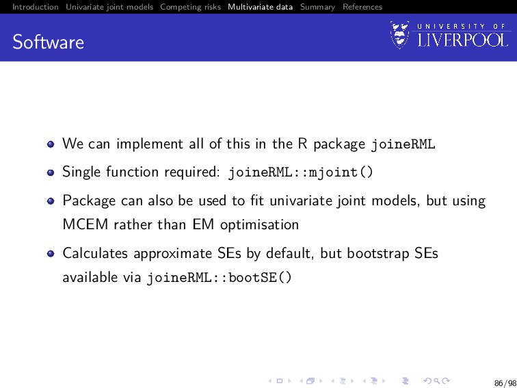
107. Introduction Univariate joint models Competing risks Multivariate data Summary References Software We can implement all of this in the R package joineRML Single function required: joineRML::mjoint() Package can also be used to fit univariate joint models, but using MCEM rather than EM optimisation Calculates approximate SEs by default, but bootstrap SEs available via joineRML::bootSE() 86/98
108. Introduction Univariate joint models Competing risks Multivariate data Summary References Proposed model for PBC data Longitudinal sub-model log(serBilir) = (β0,1 + b0i,1) + (β1,1 + b1i,1)year + εij1, albumin = (β0,2 + b0i,2) + (β1,2 + b1i,2)year + εij2, (0.1 × prothrombin)−4 = (β0,3 + b0i,3) + (β1,3 + b1i,3)year + εij3, bi ∼ N6(0, D), and εijk ∼ N(0, σ2 k ) for k = 1, 2, 3 Time-to-event sub-model λi (t) = λ0(t) exp {γv age + W2i (t)} , W2i (t) = γbil (b0i,1 + b1i,1t) + γalb (b0i,2 + b1i,2t) + γpro (b0i,3 + b1i,3t). 87/98
109. Introduction Univariate joint models Competing risks Multivariate data Summary References Example code data(pbc2) placebo <- subset(pbc2, drug == "placebo") fit.pbc <- mjoint( formLongFixed = list( "bil" = log(serBilir) ˜ year, "alb" = albumin ˜ year, "pro" = (0.1 * prothrombin)ˆ-4 ˜ year), formLongRandom = list( "bil" = ˜ year | id, "alb" = ˜ year | id, "pro" = ˜ year | id), formSurv = Surv(years, status2) ˜ age, data = placebo, timeVar = "year", control = list(tol0 = 0.001, burnin = 400)) 88/98
110. Introduction Univariate joint models Competing risks Multivariate data Summary References Results Parameter Estimate SE 95% CI β0,1 0.5541 0.0858 (0.3859, 0.7223) β1,1 0.2009 0.0201 (0.1616, 0.2402) β0,2 3.5549 0.0356 (3.4850, 3.6248) β1,2 -0.1245 0.0101 (-0.1444, -0.1047) β0,3 0.8304 0.0212 (0.7888, 0.8719) β1,3 -0.0577 0.0062 (-0.0699, -0.0456) γv 0.0462 0.0151 (0.0166, 0.0759) γbil 0.8181 0.2046 (0.4171, 1.2191) γalb -1.7060 0.6181 (-2.9173, -0.4946) γpro -2.2085 1.6070 (-5.3582, 0.9412) 89/98
111. Introduction Univariate joint models Competing risks Multivariate data Summary References Summary 90/98
112. Introduction Univariate joint models Competing risks Multivariate data Summary References Summary Joint models can be formulated to ‘link’ the ubiquitous Cox proportional hazards model and the linear mixed effects model The basic model can be extended with only slight added complexity to handle competing risks or multivariate outcomes These models can be straightforwardly fit using R 91/98
113. Introduction Univariate joint models Competing risks Multivariate data Summary References Beyond the basics Things not covered today: Alternative distributional assumptions (or lack of them) Alternative association structures How to go from fitted model to dynamic prediction Diagnostics Non-continuous longitudinal outcomes . . . It’s a rapidly growing field! 92/98
114. Introduction Univariate joint models Competing risks Multivariate data Summary References Where to find out more Univariate joint model Competing risks joint model Multivariate longitudinal data 93/98
115. Introduction Univariate joint models Competing risks Multivariate data Summary References Where to find out more 94/98
116. Introduction Univariate joint models Competing risks Multivariate data Summary References References I Henderson, Robin et al. (2000). Joint modelling of longitudinal measurements and event time data. Biostatistics 1(4), pp. 465–480. Pinheiro, Jos´ e C and Bates, Douglas M (2000). Mixed-Effects Models in S and S-PLUS. New York: Springer Verlag. Therneau, Terry M and Grambsch, Patricia M (2000). Modeling Survival Data: Extending the Cox Model. New Jersey: Springer-Verlag, p. 350. Andrinopoulou, Eleni-Rosalina et al. (2015). Combined dynamic predictions using joint models of two longitudinal outcomes and competing risk data. Statistical Methods in Medical Research 0(0), pp. 1–18. Xu, Jane and Zeger, Scott L (2001). The evaluation of multiple surrogate endpoints. Biometrics 57(1), pp. 81–87. Williamson, Paula R et al. (2008). Joint modelling of longitudinal and competing risks data. Statistics in Medicine 27, pp. 6426–6438. Wulfsohn, M S and Tsiatis, Anastasios A (1997). A joint model for survival and longitudinal data measured with error. Biometrics 53(1), pp. 330–339. 95/98
117. Introduction Univariate joint models Competing risks Multivariate data Summary References References II Laird, Nan M and Ware, James H (1982). Random-effects models for longitudinal data. Biometrics 38(4), pp. 963–74. Dempster, A P et al. (1977). Maximum likelihood from incomplete data via the EM algorithm. Journal of the Royal Statistical Society. Series B: Statistical Methodology 39(1), pp. 1–38. Hsieh, Fushing et al. (2006). Joint modeling of survival and longitudinal data: Likelihood approach revisited. Biometrics 62(4), pp. 1037–1043. Murtaugh, Paul A et al. (1994). Primary biliary cirrhosis: prediction of short-term survival based on repeated patient visits. Hepatology 20(1), pp. 126–134. Hickey, Graeme L et al. (2016). Joint modelling of time-to-event and multivariate longitudinal outcomes: recent developments and issues. BMC Medical Research Methodology 16(1), pp. 1–15. Wei, Greg C. and Tanner, Martin A. (1990). A Monte Carlo implementation of the EM algorithm and the poor man’s data augmentation algorithms. Journal of the American Statistical Association 85(411), pp. 699–704. 96/98
118. Introduction Univariate joint models Competing risks Multivariate data Summary References References III Ripatti, Samuli et al. (2002). Maximum likelihood inference for multivariate frailty models using an automated Monte Carlo EM algorithm. Lifetime Data Analysis 8(2002), pp. 349–360. McLachlan, Geoffrey J and Krishnan, Thriyambakam (2008). The EM Algorithm and Extensions. Second. Wiley-Interscience. 97/98
119. Introduction Univariate joint models Competing risks Multivariate data Summary References Next up Tea & coffee break (outside) — 1045–1100 Catch us at the break or lunch R practical session — 1100–1230 98/98