On Price Responsive Consumer Behavior in Wholesale Electricity Markets

Jaeyong An (TAMU), Grid-X Program Presentation on Day 1 (Nov.3) of Workshop on Architecture and Economics of the Future Grid

Transcript

1. On Price Responsive Consumer Behavior in Wholesale Electricity Markets Jaeyong An (Advisor: Dr. Kumar) Department of Electrical and Computer Engineering Texas A&M University November 3, 2016 1/13
2. Motivation Electricity Economically non-storable → Real-Time Commodity System objective: Real-time balancing between supply and demand Traditional Paradigm: Balancing by generation control to match volatile load Growing Penetration of Renewables: Variable Energy Resource Fluctuating over time and imperfectly predictable Limited supply controllability Demand Response (DR): The Paradigm Shift Balancing by Generation Control → Demand Control 2/13
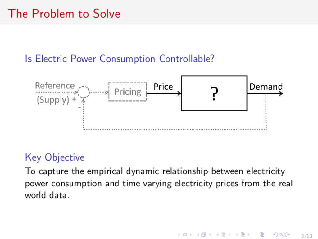
3. The Problem to Solve Is Electric Power Consumption Controllable? Key Objective To capture the empirical dynamic relationship between electricity power consumption and time varying electricity prices from the real world data. 3/13
4. Basic Approach in Our Prior Work 1 Basic Idea The dynamic modeling and control of power systems focusing on generator side is well understood. Can demand be viewed as a dynamic controllable entity like physical power system? Methodology Summary Pick an anonymous C/I customer from Houston and analyze the load and price history over nine months (Jan. 1 - Sep. 30, 2008). Transfer Function Modeling: Identify a linear dynamic model between load and price. 1J. An, P. R. Kumar, and L. Xie, “On Transfer Function Modeling of Price Responsive Demand: An Empirical Study,” in Proc. IEEE Power & Energy Society General Meeting 2015, pp. 1-5, 2015. 4/13
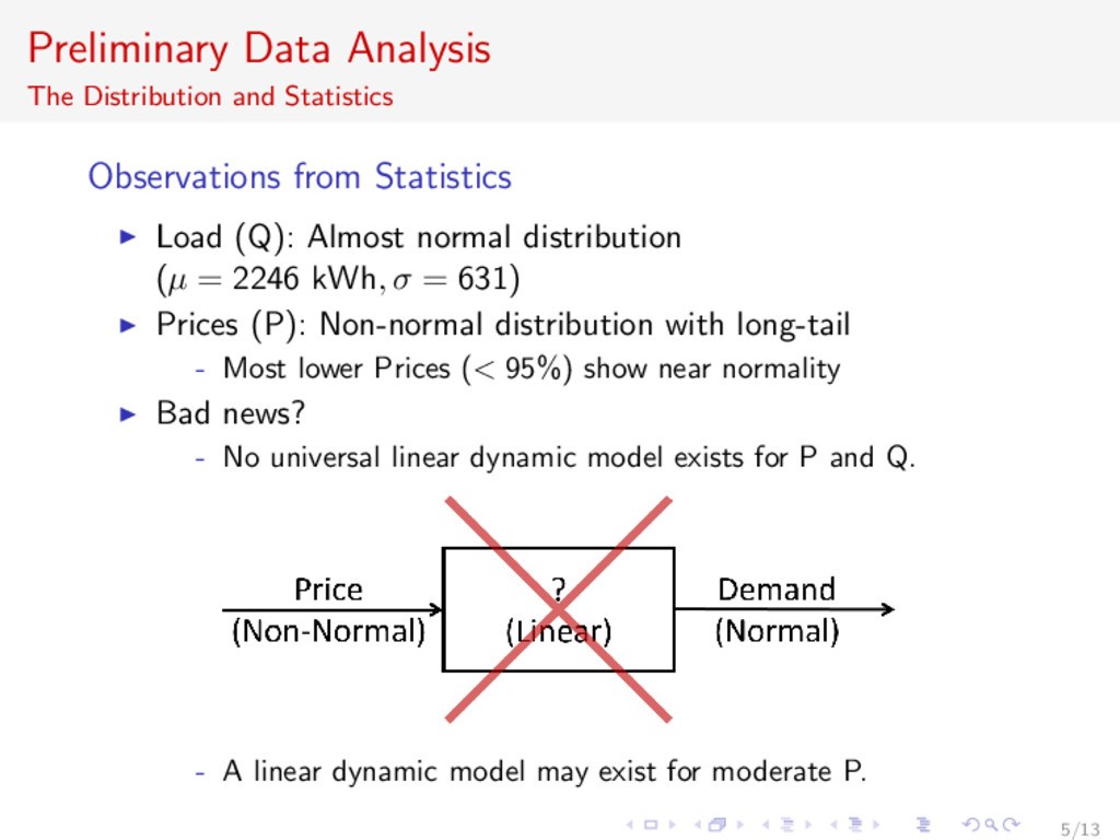
5. Preliminary Data Analysis The Distribution and Statistics Observations from Statistics Load (Q): Almost normal distribution (µ = 2246 kWh, σ = 631) Prices (P): Non-normal distribution with long-tail - Most lower Prices (< 95%) show near normality Bad news? - No universal linear dynamic model exists for P and Q. - A linear dynamic model may exist for moderate P. 5/13
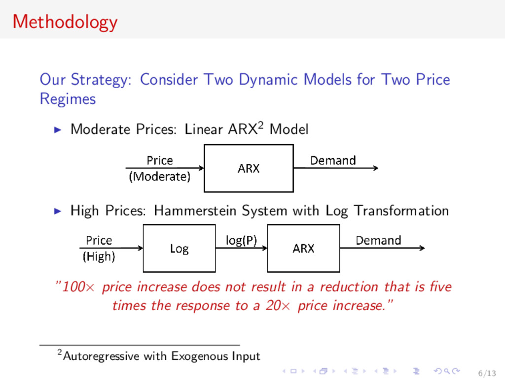
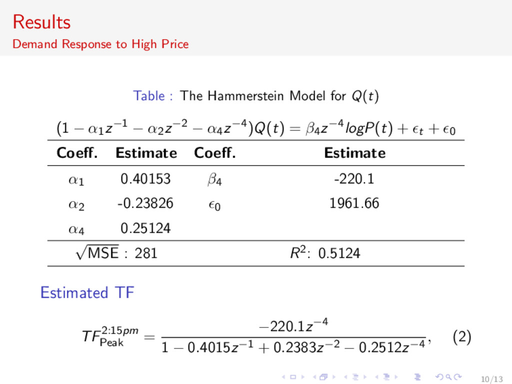
6. Methodology Our Strategy: Consider Two Dynamic Models for Two Price Regimes Moderate Prices: Linear ARX2 Model High Prices: Hammerstein System with Log Transformation ”100× price increase does not result in a reduction that is five times the response to a 20× price increase.” 2Autoregressive with Exogenous Input 6/13
7. Results Demand Response to Moderate Price Table : The ARX Model on Q(t) (1 − α1z−1 − α3z−3 − α5z−5)Q(t)(kWh) = (β1z−1 + β2z−2)P(t)($/MWh) + t + 0 Coeff. Estimate Coeff. Estimate α1 0.81268 β1 -0.8555 α3 0.046086 β2 0.5273 α5 0.036614 0 260.126 √ MSE : 301 R2: 0.776 Estimated TF TFLow = −0.8555z−1 + 0.5273z−2 1 − 0.8127z−1 − 0.0461z−3 − 0.0366z−5 . (1) 7/13
8. Results Demand Response to High Price 15 15.5 16 16.5 17 17.5 18 0 200 400 600 800 1000 Time (hour) Price ($/MWh) Sample Price Spike (Apr. 3) 15 15.5 16 16.5 17 17.5 18 800 1000 1200 1400 1600 Time (hour) Load (kWh) Sample Demand Response (Apr. 3) (a) 3:30pm Apr. 3, 2008. 0 0.25 0.5 0.75 1 1.25 1.5 1.75 2 2.25 2.5 500 1000 1500 2000 2500 3000 3500 4000 lag (hour) Q (kWh) (b) The box plot of Q after a price surge (over 95%-quantile) at lag=0. (1:00 PM - 4:00 PM) 8/13
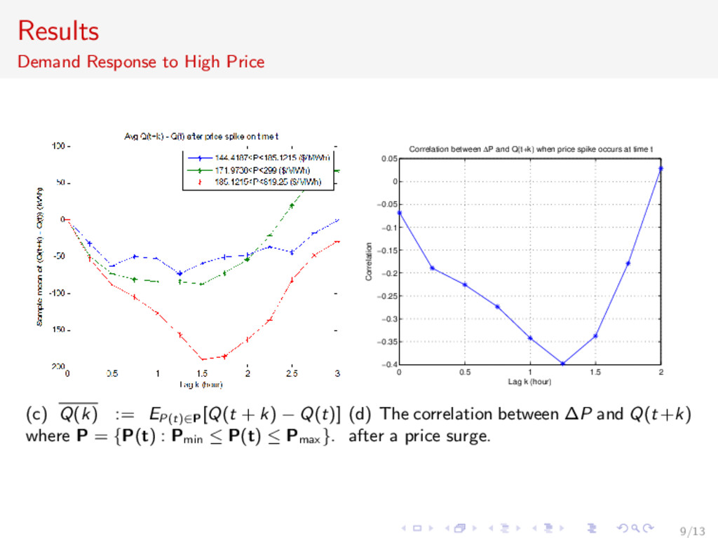
9. Results Demand Response to High Price (c) Q(k) := EP(t)∈P [Q(t + k) − Q(t)] where P = {P(t) : Pmin ≤ P(t) ≤ Pmax}. 0 0.5 1 1.5 2 −0.4 −0.35 −0.3 −0.25 −0.2 −0.15 −0.1 −0.05 0 0.05 Correlation between ∆P and Q(t+k) when price spike occurs at time t Lag k (hour) Correlation (d) The correlation between ∆P and Q(t+k) after a price surge. 9/13
10. Results Demand Response to High Price Table : The Hammerstein Model for Q(t) (1 − α1z−1 − α2z−2 − α4z−4)Q(t) = β4z−4logP(t) + t + 0 Coeff. Estimate Coeff. Estimate α1 0.40153 β4 -220.1 α2 -0.23826 0 1961.66 α4 0.25124 √ MSE : 281 R2: 0.5124 Estimated TF TF2:15pm Peak = −220.1z−4 1 − 0.4015z−1 + 0.2383z−2 − 0.2512z−4 , (2) 10/13
11. Wrap-Up Summary We proposed a nonlinear dynamical system approach for modeling price responsive electricity demand. Conclusion The price responsiveness of demand has qualitatively different behavior during normal price and peak price periods. - A moderate price has very little impact with respect to eliciting demand response. - A price spike has a considerable but delayed impact in eliciting demand response. Future Works Design of effective pricing to close loop around demand response. 11/13
12. Appendices 12/13
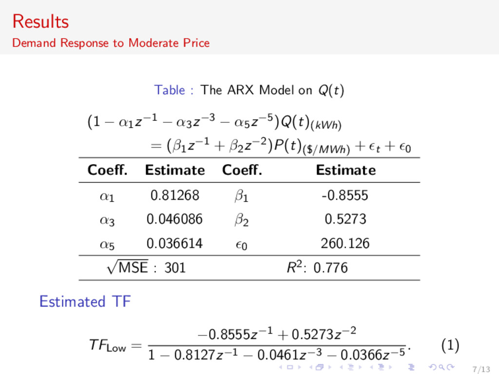
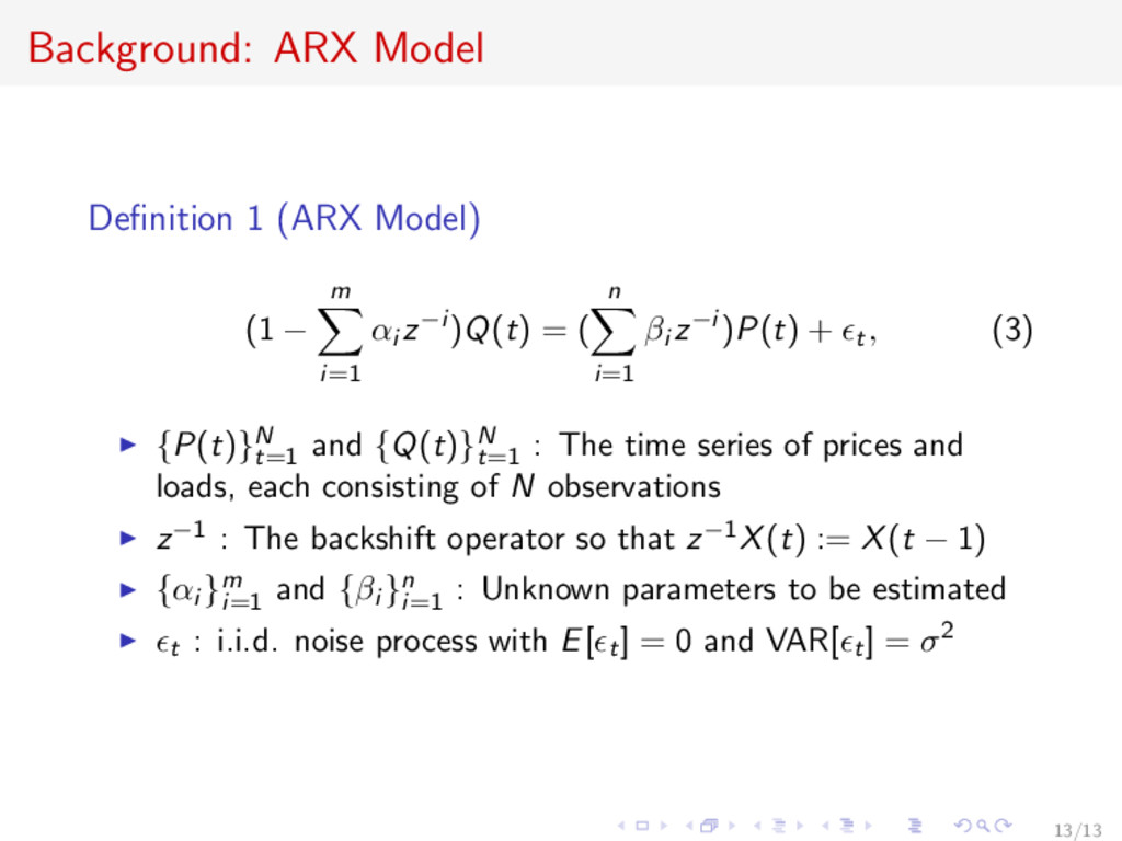
13. Background: ARX Model Definition 1 (ARX Model) (1 − m i=1 αi z−i )Q(t) = ( n i=1 βi z−i )P(t) + t, (3) {P(t)}N t=1 and {Q(t)}N t=1 : The time series of prices and loads, each consisting of N observations z−1 : The backshift operator so that z−1X(t) := X(t − 1) {αi }m i=1 and {βi }n i=1 : Unknown parameters to be estimated t : i.i.d. noise process with E[ t] = 0 and VAR[ t] = σ2 13/13