Lecture slides for POM 1-14

生産管理技術1の講義14のスライドです．

Transcript

1. © Hajime Mizuyama Production & Operations Management #1 @AGU Lec.14: Job Shop Scheduling • Job shop scheduling problem • Graphical approach to two-job case • Dispatching rules and rule-based scheduling
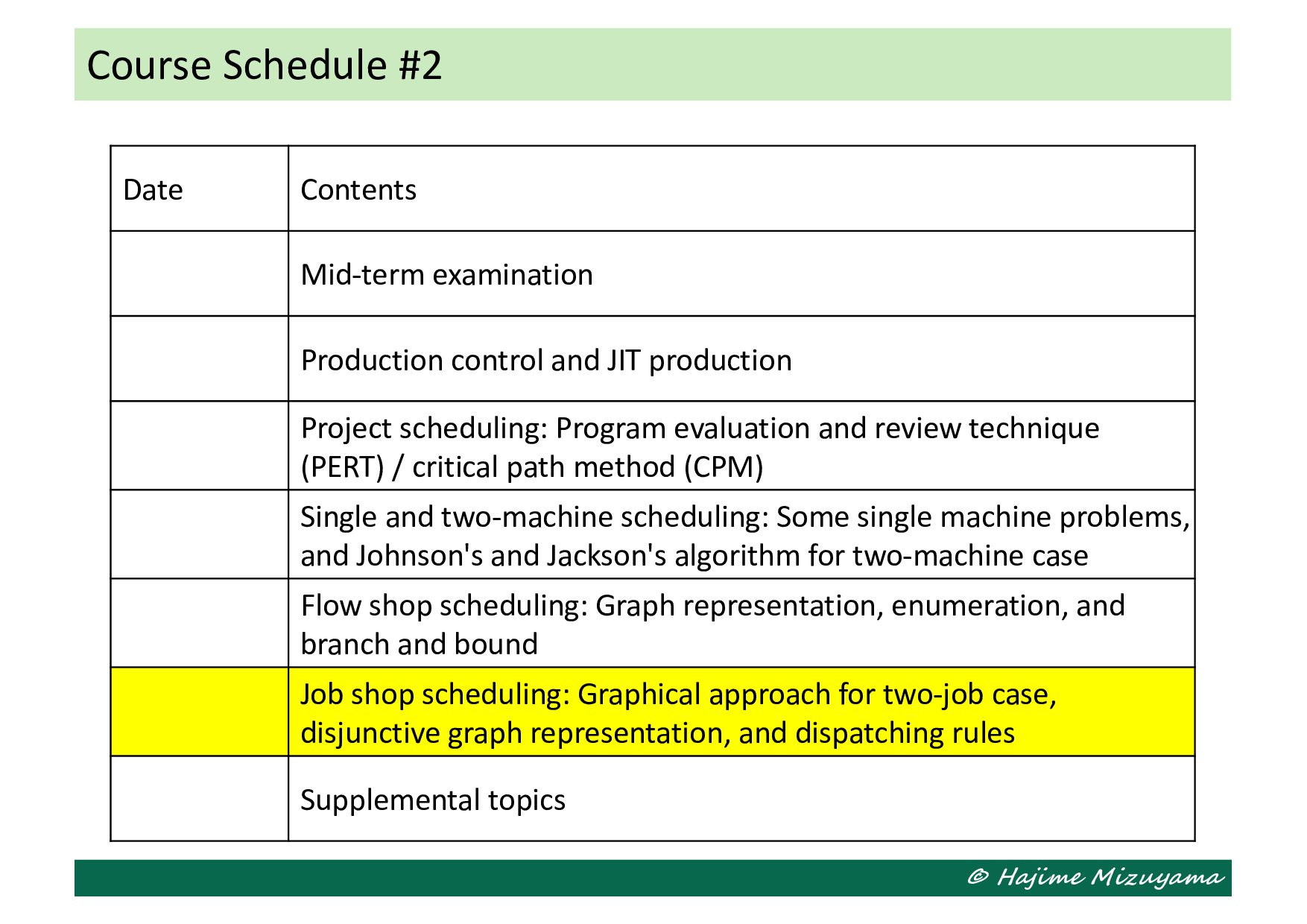
2. © Hajime Mizuyama Course Schedule #2 Date Contents Mid-term examination Production control and JIT production Project scheduling: Program evaluation and review technique (PERT) / critical path method (CPM) Single and two-machine scheduling: Some single machine problems, and Johnson's and Jackson's algorithm for two-machine case Flow shop scheduling: Graph representation, enumeration, and branch and bound Job shop scheduling: Graphical approach for two-job case, disjunctive graph representation, and dispatching rules Supplemental topics
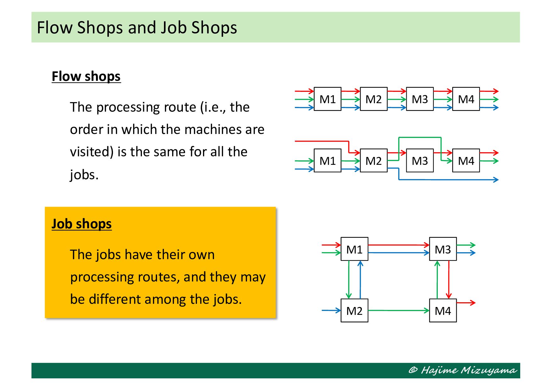
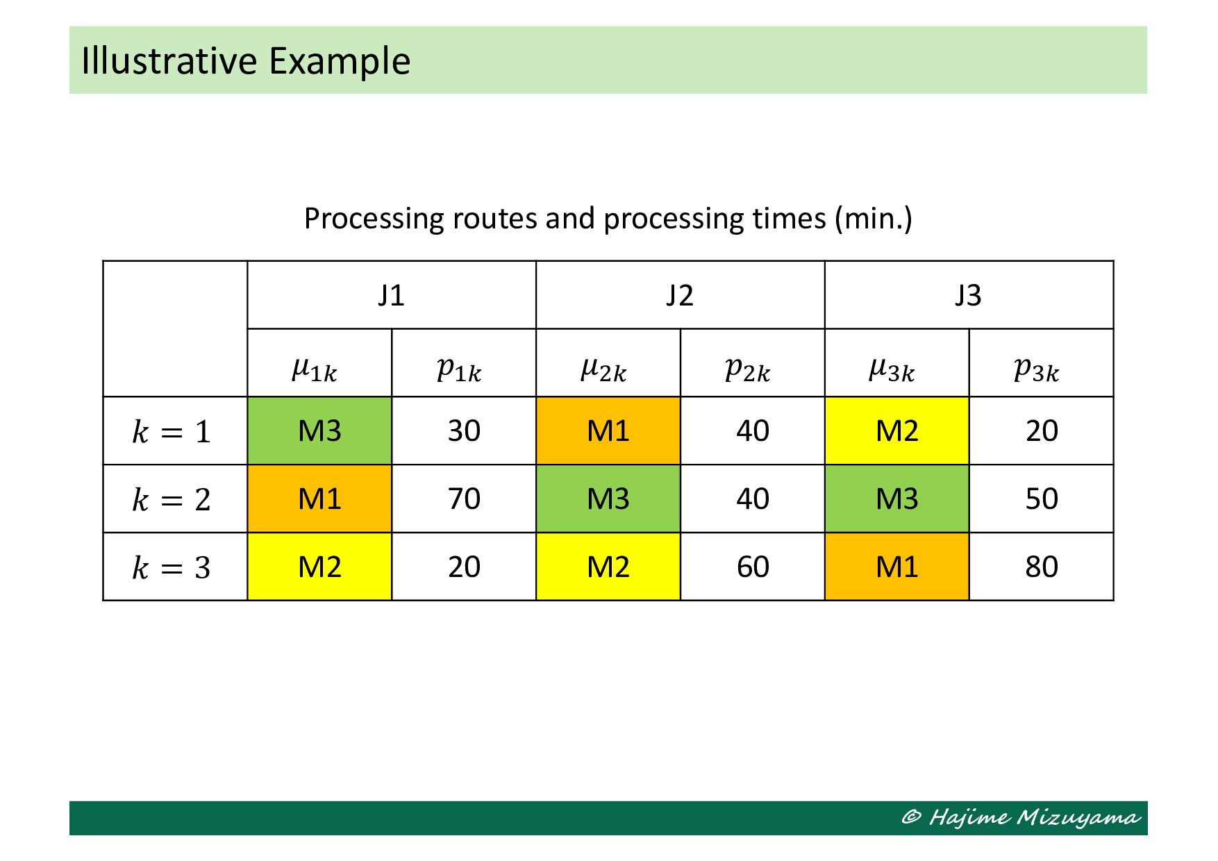
3. © Hajime Mizuyama Flow Shops and Job Shops Flow shops The processing route (i.e., the order in which the machines are visited) is the same for all the jobs. Job shops The jobs have their own processing routes, and they may be different among the jobs. M1 M2 M3 M4 M1 M2 M3 M4 M1 M2 M3 M4
4. © Hajime Mizuyama There are multiple machines and jobs with different processing routes. The jobs on each machine should be ordered to minimize the makespan. • Job set and machine set: 𝐽 = {1, 2, … , |𝐽|} and 𝑀 = {1, 2, … , |𝑀|} • Set of operations of job 𝑗 ∈ 𝐽: 𝐾! " = { 𝑗, 1 , 𝑗, 2 , … , (𝑗, |𝐾! "|)} • Processing time of operation (𝑗, 𝑘) ∈ 𝐾! ": 𝑝!# • Machine carrying out operation (𝑗, 𝑘) ∈ 𝐾! " : 𝜇!# ∈ 𝑀 • Set of operations on machine 𝑚 ∈ 𝑀: (𝑗, 𝑘) 𝜇!# = 𝑚} ≡ 𝐾$ % • Operation sequence on machine 𝑚 ∈ 𝑀: 𝜋$ = (𝜋$& , 𝜋$' , … , 𝜋$ (! " ) • Starting and completion times of operation (𝑗, 𝑘) ∈ 𝐾! ": 𝑆!# and 𝐶!# • Makespan: 𝐶)*+ = max (!,#)∈(# $ 𝐶!# Job Shop Scheduling Problem
5. © Hajime Mizuyama J1 J2 J3 𝜇&# 𝑝&# 𝜇'# 𝑝'# 𝜇0# 𝑝0# 𝑘 = 1 M3 30 M1 40 M2 20 𝑘 = 2 M1 70 M3 40 M3 50 𝑘 = 3 M2 20 M2 60 M1 80 Illustrative Example Processing routes and processing times (min.)
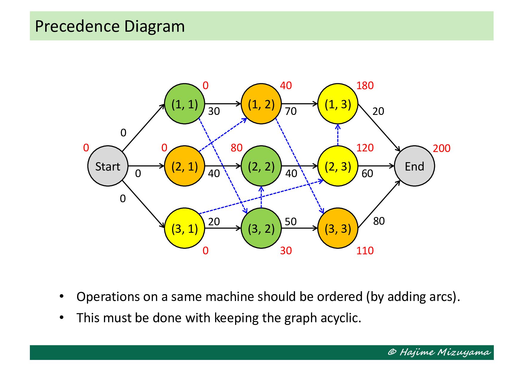
6. © Hajime Mizuyama Precedence Diagram Start (1, 1) (2, 1) (3, 1) (1, 2) (2, 2) (3, 2) (1, 3) (2, 3) (3, 3) End • Operations on a same machine should be ordered (by adding arcs). • This must be done with keeping the graph acyclic. 0 0 0 30 40 20 70 40 50 20 60 80
7. © Hajime Mizuyama Precedence Diagram Start (1, 1) (2, 1) (3, 1) (1, 2) (2, 2) (3, 2) (1, 3) (2, 3) (3, 3) 0 0 0 30 40 20 70 40 50 0 40 180 0 0 80 120 0 30 110 End 200 20 60 80 • Operations on a same machine should be ordered (by adding arcs). • This must be done with keeping the graph acyclic.
8. © Hajime Mizuyama J2 J1 J3 Corresponding Schedule M1 M2 M3 J1 J1 J2 J2 J3 J3
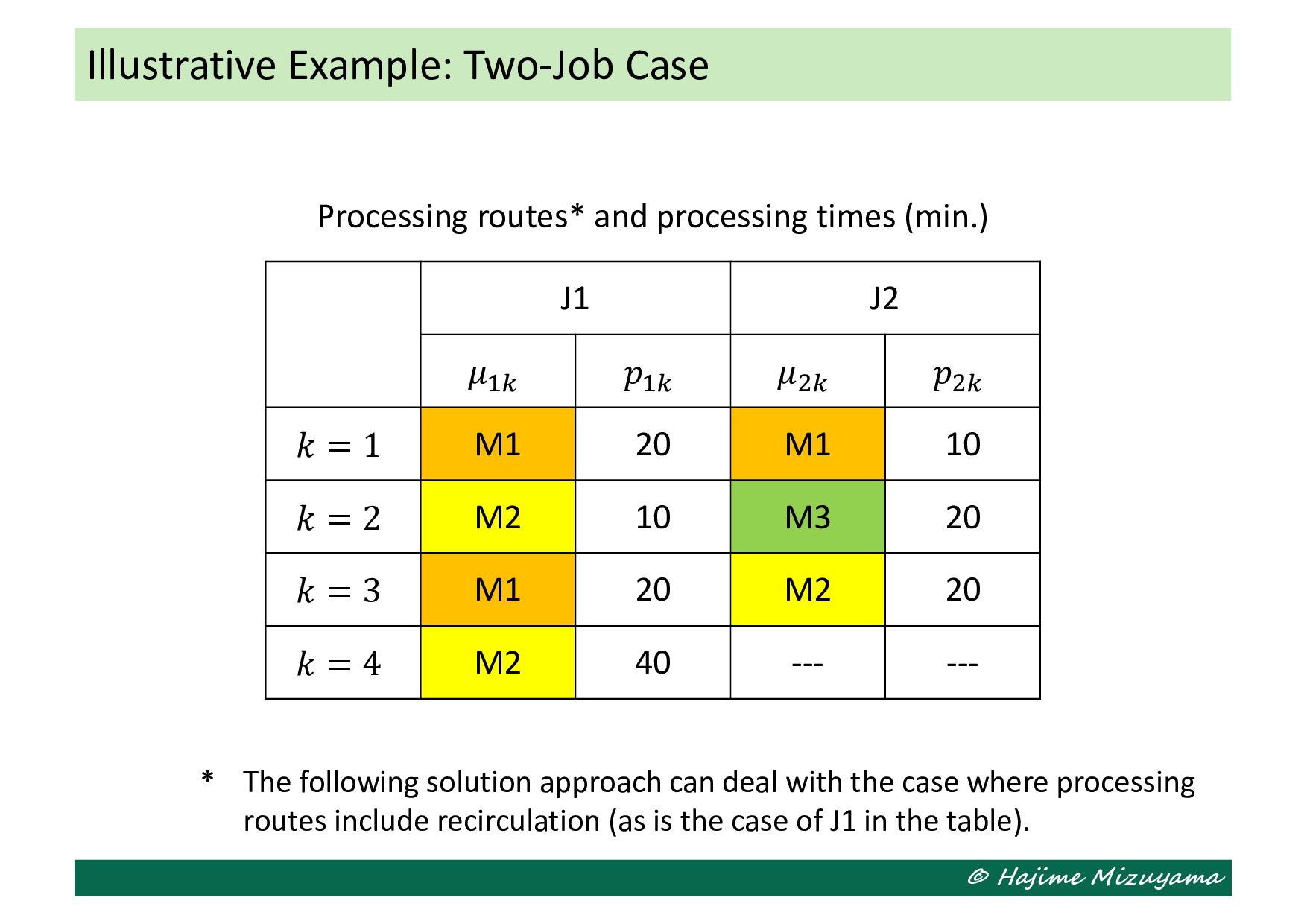
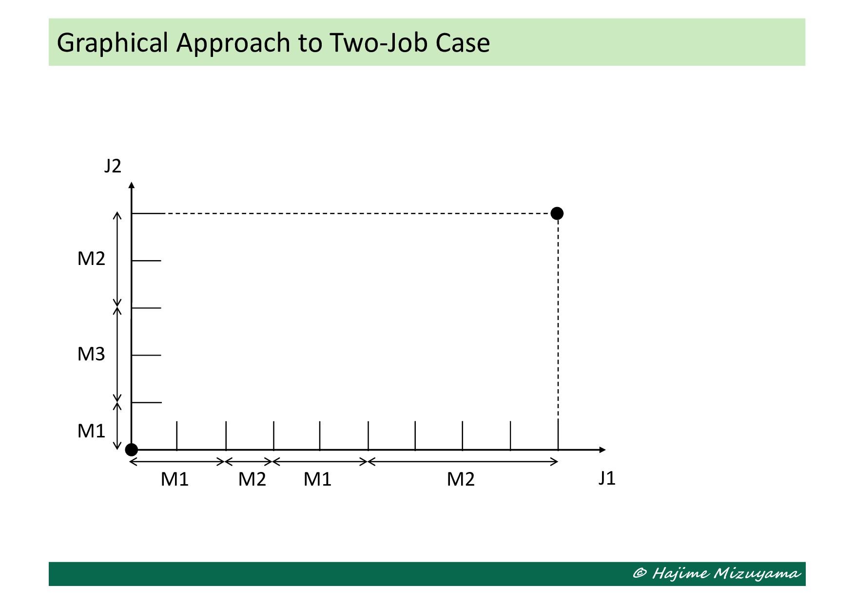
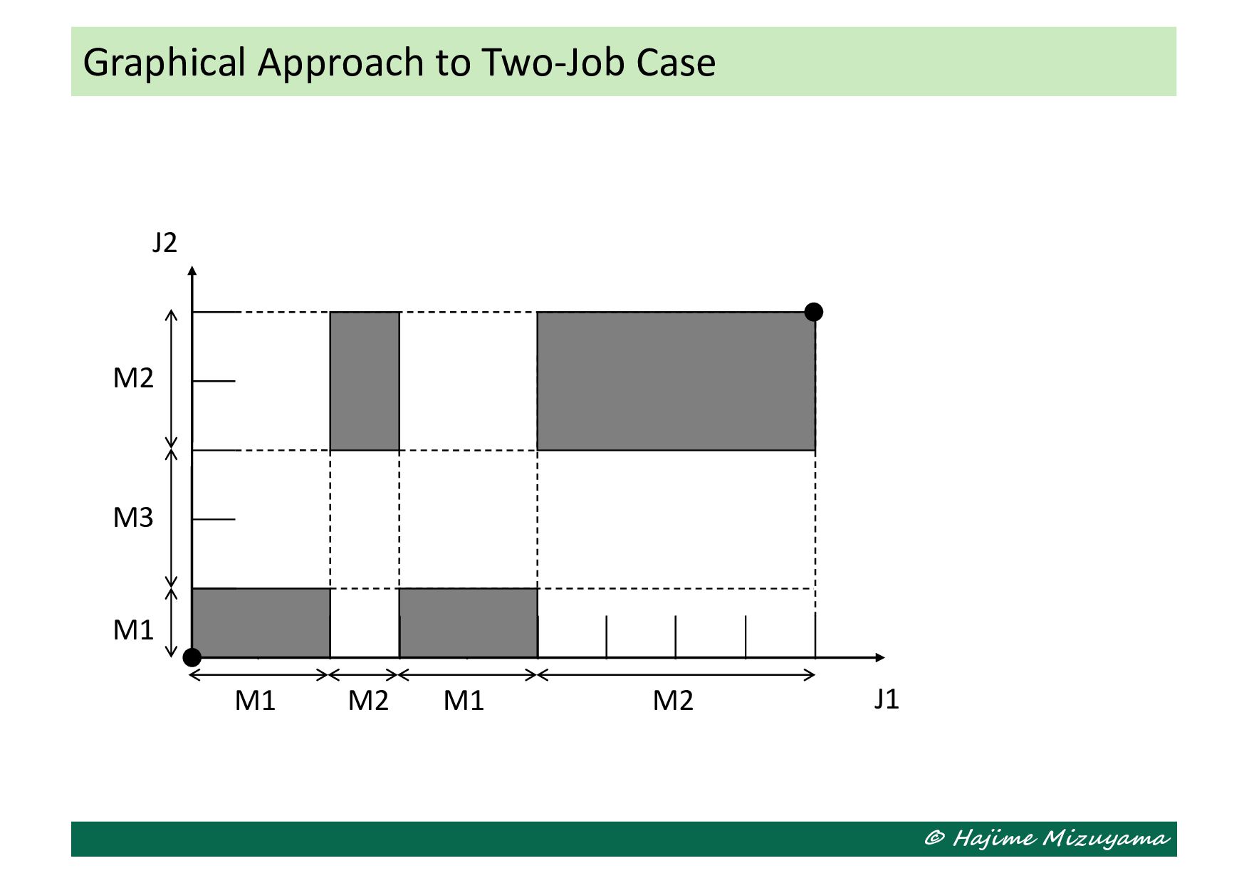
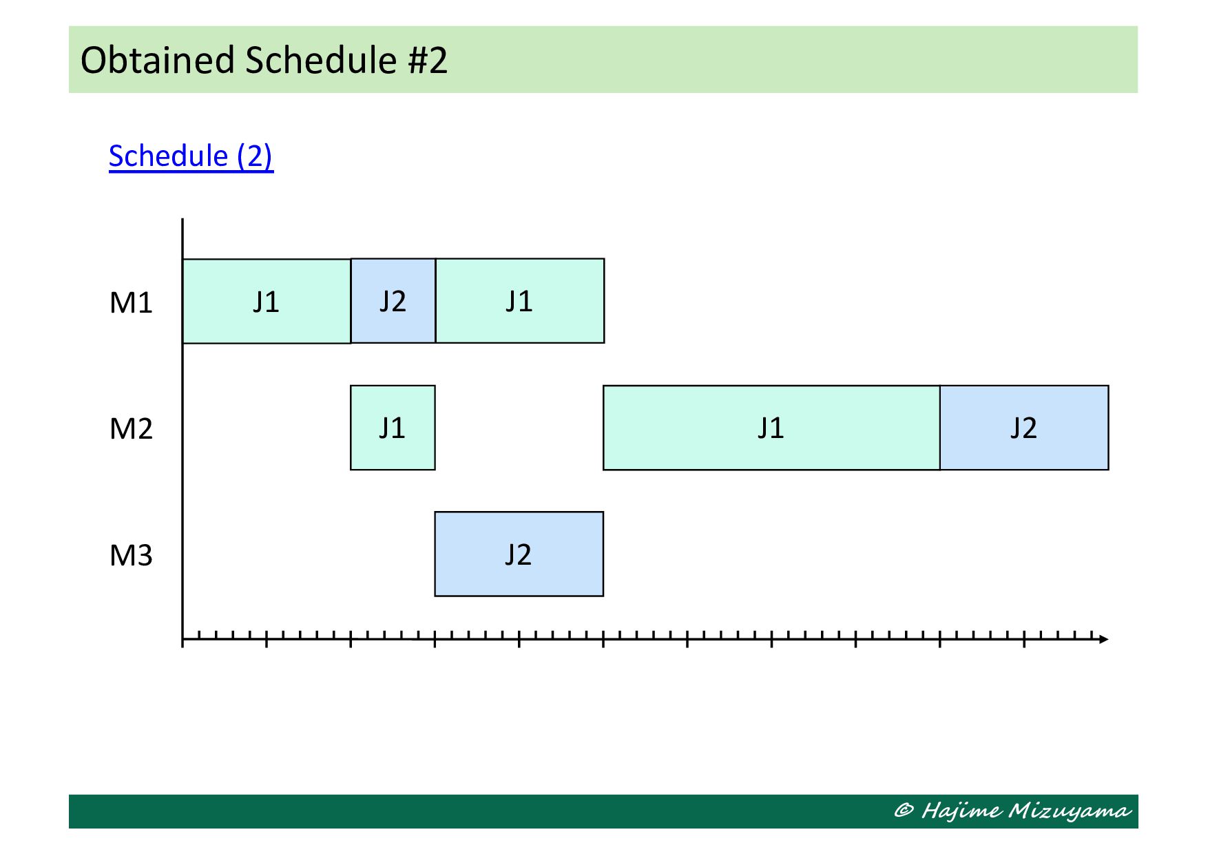
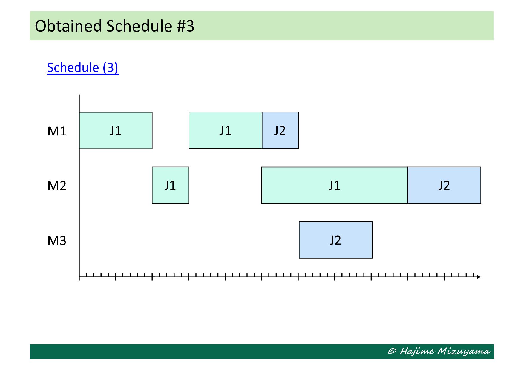
9. © Hajime Mizuyama J1 J2 𝜇&# 𝑝&# 𝜇'# 𝑝'# 𝑘 = 1 M1 20 M1 10 𝑘 = 2 M2 10 M3 20 𝑘 = 3 M1 20 M2 20 𝑘 = 4 M2 40 --- --- Illustrative Example: Two-Job Case Processing routes* and processing times (min.) * The following solution approach can deal with the case where processing routes include recirculation (as is the case of J1 in the table).
10. © Hajime Mizuyama Graphical Approach to Two-Job Case M3 M2 M1 J1 J2 M1 M2 M1 M2
11. © Hajime Mizuyama Graphical Approach to Two-Job Case M3 M2 M1 M1 M2 M1 M2 J1 J2
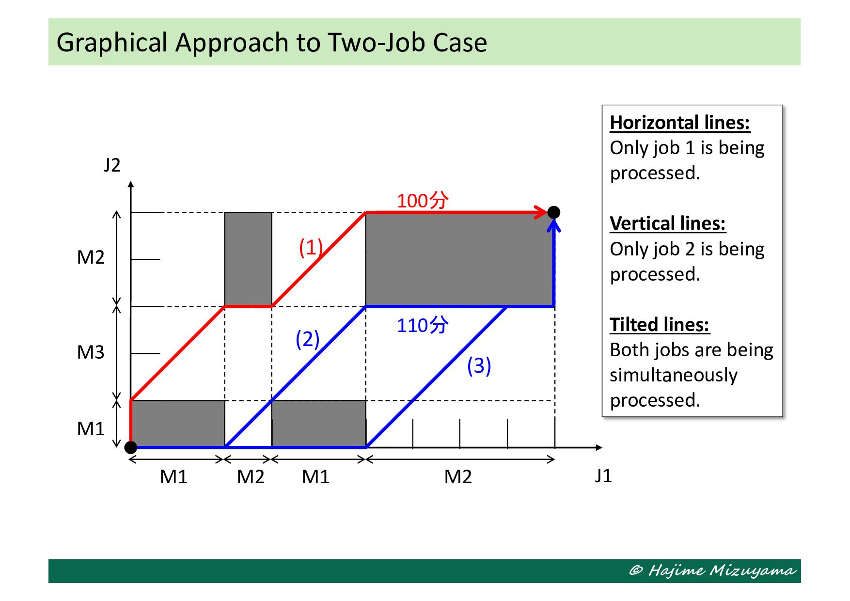
12. © Hajime Mizuyama Graphical Approach to Two-Job Case M3 M2 M1 Horizontal lines: Only job 1 is being processed. Vertical lines: Only job 2 is being processed. Tilted lines: Both jobs are being simultaneously processed. 100分 110分 M1 M2 M1 M2 (1) (2) (3) J1 J2
13. © Hajime Mizuyama Obtained Schedule #1 M1 M2 J2 J1 M3 J1 J1 J1 J2 J2 Schedule (1)
14. © Hajime Mizuyama Obtained Schedule #2 M1 M2 J2 J1 M3 J1 J1 J1 J2 J2 Schedule (2)
15. © Hajime Mizuyama Obtained Schedule #3 M1 M2 J2 J1 M3 J1 J1 J1 J2 J2 Schedule (3)
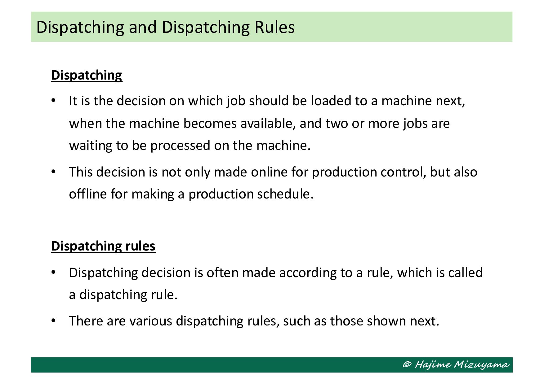
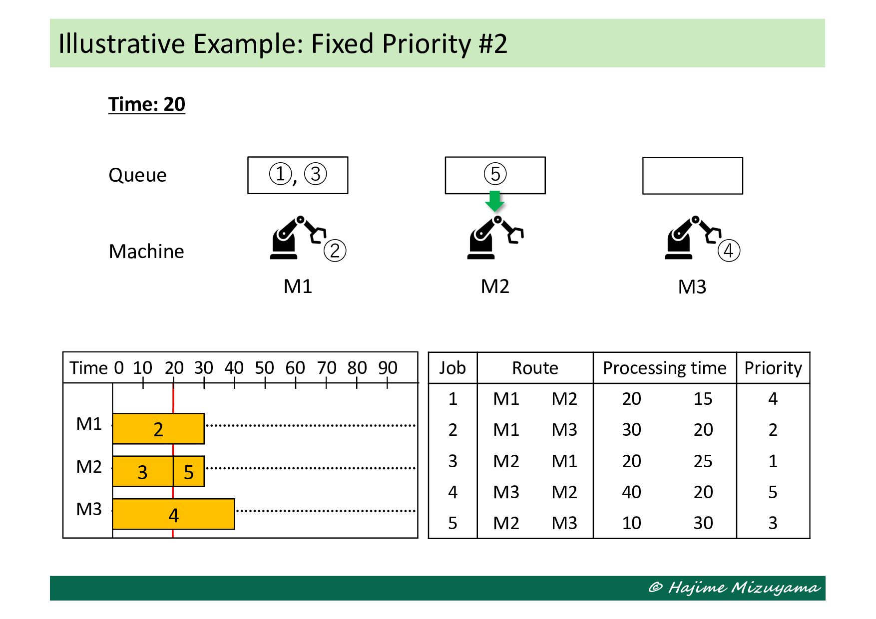
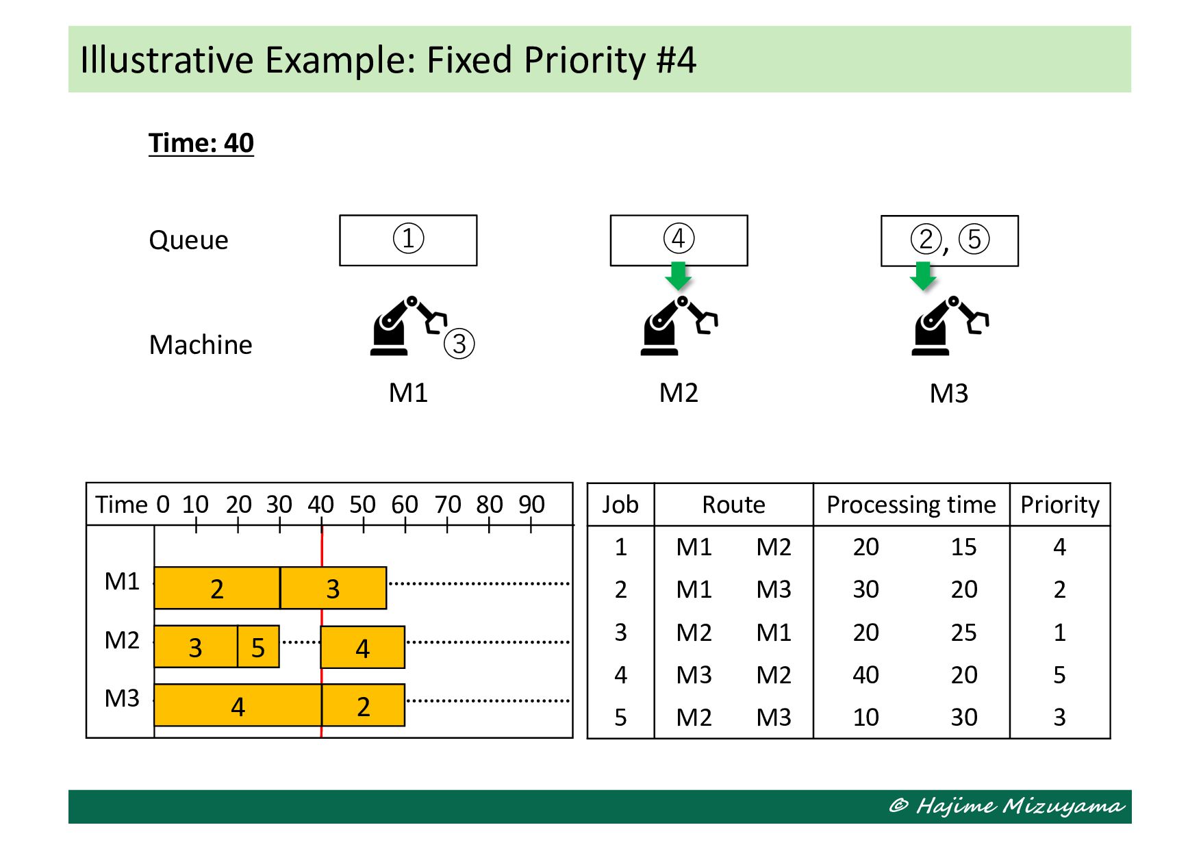
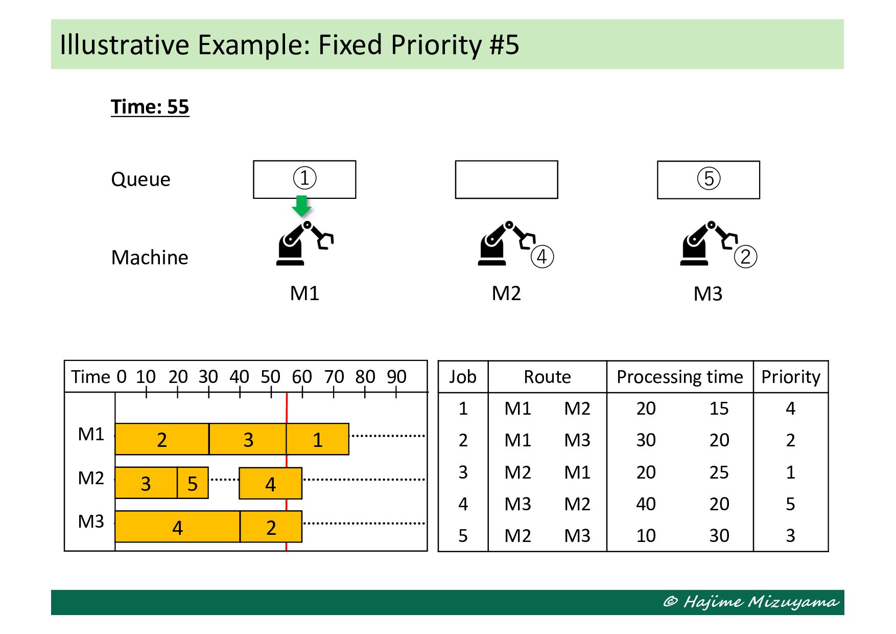
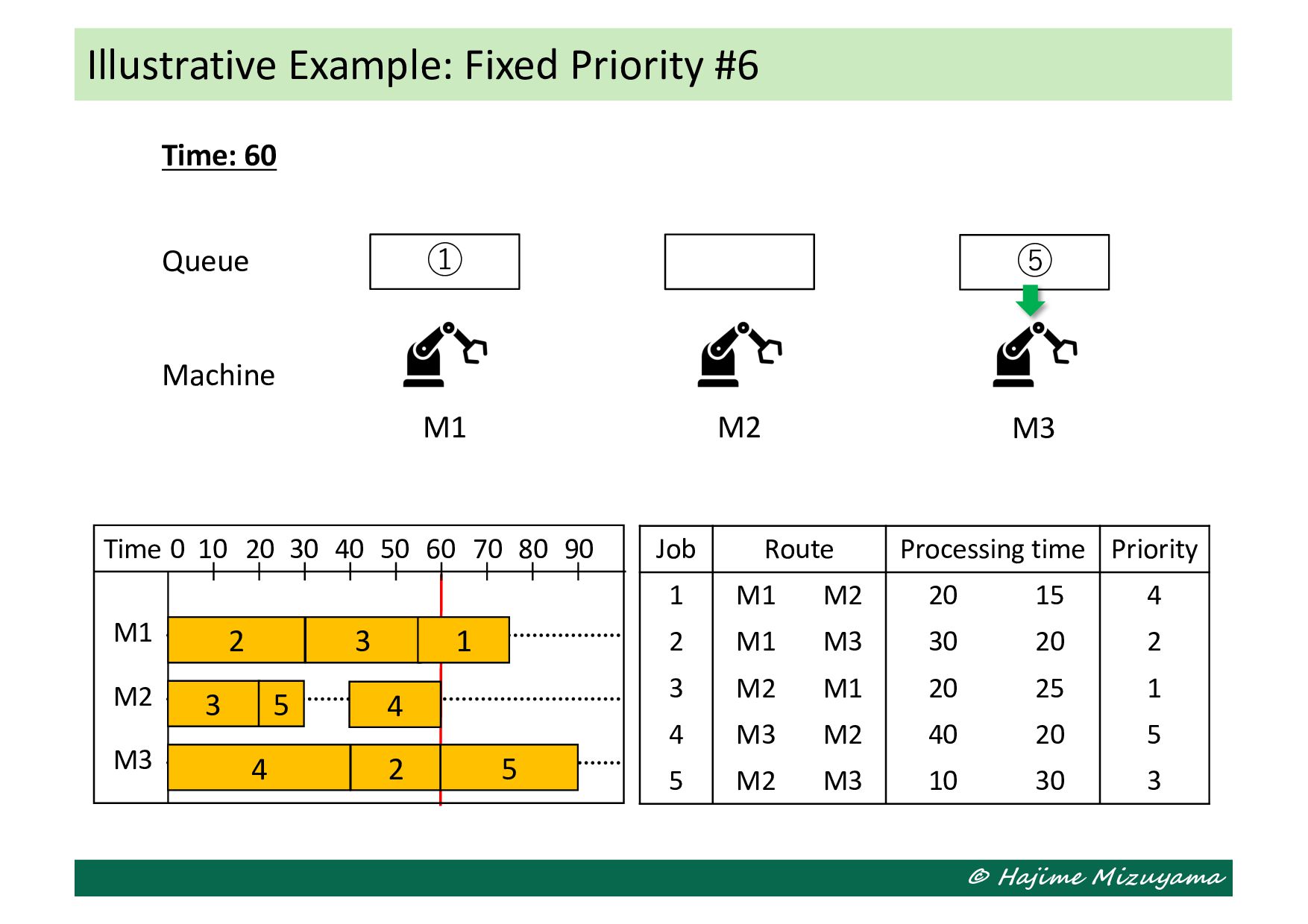
16. © Hajime Mizuyama Dispatching • It is the decision on which job should be loaded to a machine next, when the machine becomes available, and two or more jobs are waiting to be processed on the machine. • This decision is not only made online for production control, but also offline for making a production schedule. Dispatching rules • Dispatching decision is often made according to a rule, which is called a dispatching rule. • There are various dispatching rules, such as those shown next. Dispatching and Dispatching Rules
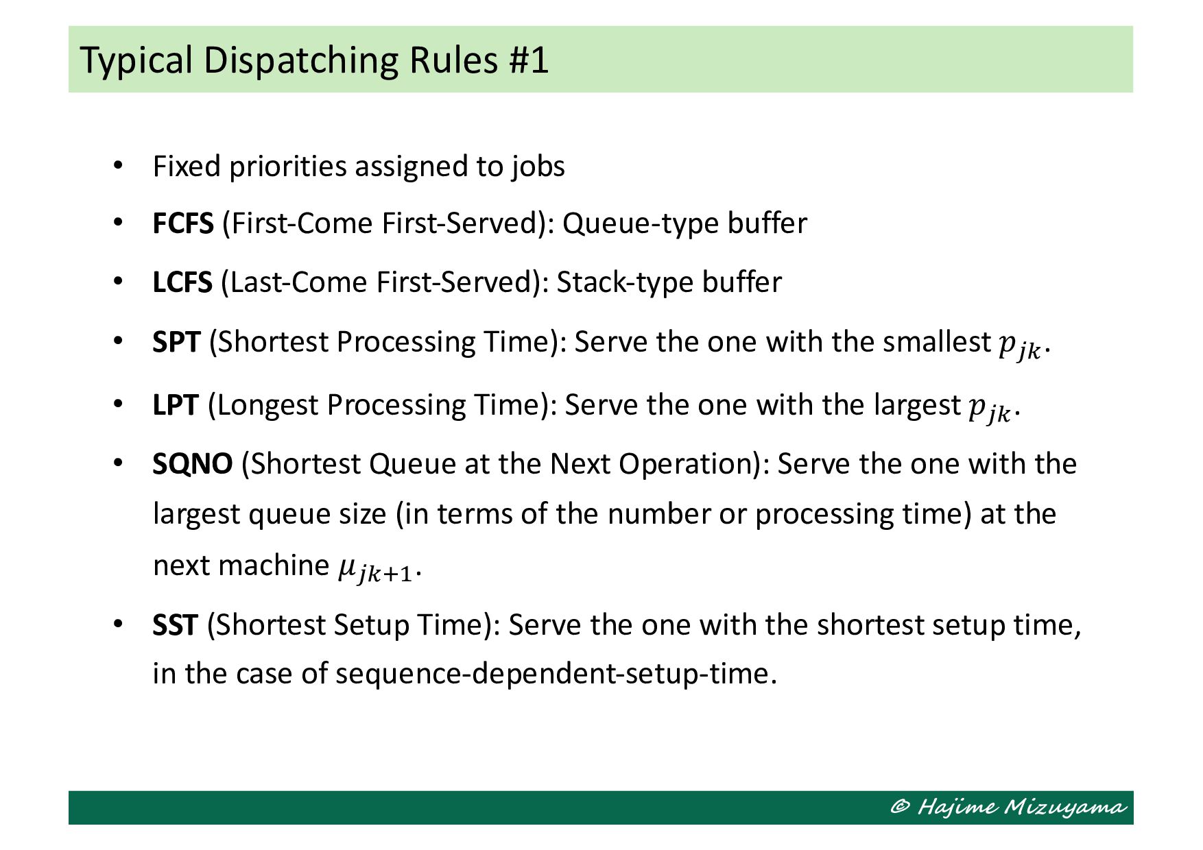
17. © Hajime Mizuyama • Fixed priorities assigned to jobs • FCFS (First-Come First-Served): Queue-type buffer • LCFS (Last-Come First-Served): Stack-type buffer • SPT (Shortest Processing Time): Serve the one with the smallest 𝑝!#. • LPT (Longest Processing Time): Serve the one with the largest 𝑝!#. • SQNO (Shortest Queue at the Next Operation): Serve the one with the largest queue size (in terms of the number or processing time) at the next machine 𝜇!#1&. • SST (Shortest Setup Time): Serve the one with the shortest setup time, in the case of sequence-dependent-setup-time. Typical Dispatching Rules #1
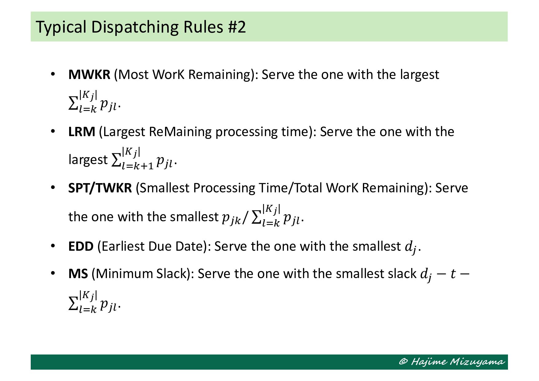
18. © Hajime Mizuyama • MWKR (Most WorK Remaining): Serve the one with the largest ∑ 23# |(#| 𝑝!2. • LRM (Largest ReMaining processing time): Serve the one with the largest ∑ 23#1& |(#| 𝑝!2. • SPT/TWKR (Smallest Processing Time/Total WorK Remaining): Serve the one with the smallest 𝑝!# / ∑ 23# |(#| 𝑝!2. • EDD (Earliest Due Date): Serve the one with the smallest 𝑑!. • MS (Minimum Slack): Serve the one with the smallest slack 𝑑! − 𝑡 − ∑ 23# |(#| 𝑝!2. Typical Dispatching Rules #2
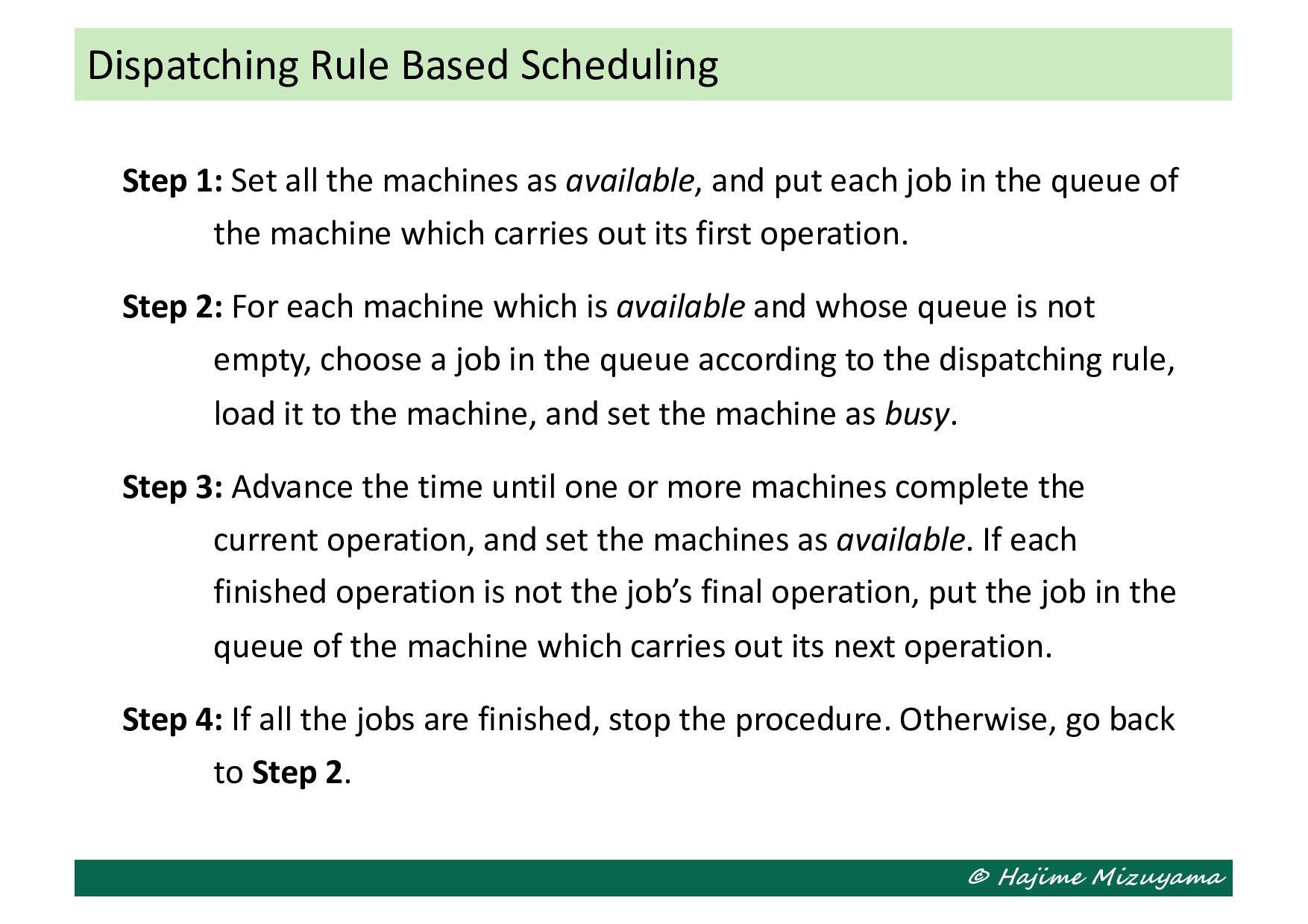
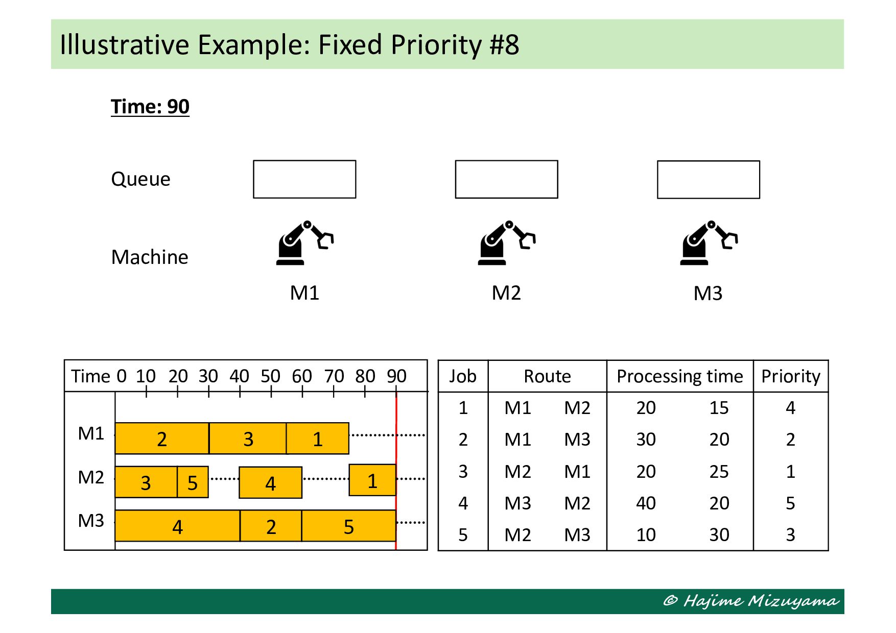
19. © Hajime Mizuyama Step 1: Set all the machines as available, and put each job in the queue of the machine which carries out its first operation. Step 2: For each machine which is available and whose queue is not empty, choose a job in the queue according to the dispatching rule, load it to the machine, and set the machine as busy. Step 3: Advance the time until one or more machines complete the current operation, and set the machines as available. If each finished operation is not the job’s final operation, put the job in the queue of the machine which carries out its next operation. Step 4: If all the jobs are finished, stop the procedure. Otherwise, go back to Step 2. Dispatching Rule Based Scheduling
20. © Hajime Mizuyama Processing route Processing time (min.) Priority 𝜇!" 𝜇!# 𝑝!" 𝑝!# J1 M1 M2 20 15 2 J2 M1 M3 30 20 1 J3 M2 M1 20 25 3 J4 M3 M2 40 20 5 J5 M2 M3 10 30 4 Illustrative Example
21. © Hajime Mizuyama Illustrative Example: Fixed Priority #1 Time: 0 M1 M2 M3 Job Route Processing time Priority 1 M1 M2 20 15 4 2 M1 M3 30 20 2 3 M2 M1 20 25 1 4 M3 M2 40 20 5 5 M2 M3 10 30 3 ①, ② ③, ⑤ ④ Queue Machine 10 20 30 40 50 0 M1 M2 M3 60 70 80 90 Time 4 2 3
22. © Hajime Mizuyama Illustrative Example: Fixed Priority #2 Time: 20 M1 M2 M3 Job Route Processing time Priority 1 M1 M2 20 15 4 2 M1 M3 30 20 2 3 M2 M1 20 25 1 4 M3 M2 40 20 5 5 M2 M3 10 30 3 ①, ③ ⑤ Queue Machine 10 20 30 40 50 0 M1 M2 M3 60 70 80 90 Time 4 2 3 ② ④ 5
23. © Hajime Mizuyama Illustrative Example: Fixed Priority #3 Time: 30 M1 M2 M3 Job Route Processing time Priority 1 M1 M2 20 15 4 2 M1 M3 30 20 2 3 M2 M1 20 25 1 4 M3 M2 40 20 5 5 M2 M3 10 30 3 ①, ③ ②, ⑤ Queue Machine 10 20 30 40 50 0 M1 M2 M3 60 70 80 90 Time 4 2 3 ④ 5 3
24. © Hajime Mizuyama Illustrative Example: Fixed Priority #4 Time: 40 M1 M2 M3 Job Route Processing time Priority 1 M1 M2 20 15 4 2 M1 M3 30 20 2 3 M2 M1 20 25 1 4 M3 M2 40 20 5 5 M2 M3 10 30 3 ① ④ ②, ⑤ Queue Machine 10 20 30 40 50 0 M1 M2 M3 60 70 80 90 Time 4 2 3 5 3 ③ 4 2
25. © Hajime Mizuyama Illustrative Example: Fixed Priority #5 Time: 55 M1 M2 M3 Job Route Processing time Priority 1 M1 M2 20 15 4 2 M1 M3 30 20 2 3 M2 M1 20 25 1 4 M3 M2 40 20 5 5 M2 M3 10 30 3 ① ⑤ Queue Machine 10 20 30 40 50 0 M1 M2 M3 60 70 80 90 Time 4 2 3 5 3 ④ 4 2 ② 1
26. © Hajime Mizuyama Illustrative Example: Fixed Priority #6 Time: 60 M1 M2 M3 Job Route Processing time Priority 1 M1 M2 20 15 4 2 M1 M3 30 20 2 3 M2 M1 20 25 1 4 M3 M2 40 20 5 5 M2 M3 10 30 3 ① ⑤ Queue Machine 10 20 30 40 50 0 M1 M2 M3 60 70 80 90 Time 4 2 3 5 3 4 2 1 5
27. © Hajime Mizuyama Illustrative Example: Fixed Priority #7 Time: 75 M1 M2 M3 Job Route Processing time Priority 1 M1 M2 20 15 4 2 M1 M3 30 20 2 3 M2 M1 20 25 1 4 M3 M2 40 20 5 5 M2 M3 10 30 3 ① Queue Machine 10 20 30 40 50 0 M1 M2 M3 60 70 80 90 Time 4 2 3 5 3 4 2 1 5 ⑤ 1
28. © Hajime Mizuyama Illustrative Example: Fixed Priority #8 Time: 90 M1 M2 M3 Job Route Processing time Priority 1 M1 M2 20 15 4 2 M1 M3 30 20 2 3 M2 M1 20 25 1 4 M3 M2 40 20 5 5 M2 M3 10 30 3 Queue Machine 10 20 30 40 50 0 M1 M2 M3 60 70 80 90 Time 4 2 3 5 3 4 2 1 5 1