Lecture slides for POM 1-8

生産管理技術1の講義8のスライドです．

Transcript

1. © Hajime Mizuyama Production & Operations Management #1 @AGU Lec.8: MRP (2) • Lot sizing and dynamic order quantity (DOQ) • Various approaches to lot sizing • Wagner-Whitin method (WW method)
2. © Hajime Mizuyama Course Schedule #1 Date Contents Outline of production management (1): How to conceptualize production systems Outline of production management (2): Framework of production planning and control Inventory control and management (1): Economic order quantity (EOQ) and the role of safety stock Inventory control and management (2): Conventional inventory control models Production planning and linear programming MRP (1): Bill of materials (BOM), priority planning, capacity planning, etc. MRP (2): Lot sizing and dynamic order quantity (DOQ)
3. © Hajime Mizuyama • The net requirements calculated by naïve priority planning may not be the most economical way of forming production lots (or orders). • It is sometime more economical to group some consecutive small size requirements into a single production lot (or order). • Because it reduces the setup cost, which are proportional to the number of periods where production is carried out. • Let’s minimize the sum of the setup cost and inventory holding cost under the constraint that all the requirements should be satisfied. Appropriate lot (re)formation Necessity of Lot Sizing
4. © Hajime Mizuyama Lot for lot The net requirement in each period is treated as a separate order. Fixed order quantity Use the same lot size for every order, for example, EOQ. Fixed order cycle The net requirements for a specified number of consecutive periods are grouped together into an order. Wagner-Whitin (WW) method Lot sizes are determined dynamically to minimize the total cost. Approaches to Lot Sizing
5. © Hajime Mizuyama • Planning horizon (periods): 𝑡 ∈ {1, 2, … , 𝑁} • Net requirement in period 𝑡: 𝐷! • Setup cost incurred if production is carried out in period 𝑡: 𝐴! • Inventory holding cost per item per period: ℎ • Indicator of whether production is carried out in period 𝑡: 𝑋! ∈ {0, 1} • Lot number fulfilling the requirement in period 𝑡: 𝐿! (𝑋) = ∑"#$ ! 𝑋! • Lot size (order quantity) of production lot 𝑙: 𝑄% (𝑋) = ∑!∈{"|)!(+)#%} 𝐷! • The period when production lot 𝑙 is produced: 𝑇% (𝑋) = min !∈{"|)!(+)#%} 𝑡 • Total costs to be minimized: ∑!#$ . [𝐴! ; 𝑋! + ℎ ; (𝑡 − 𝑇)"(+) (𝑋)) ; 𝐷! ] Notation For simplicity, lead-time is not considered here.
6. © Hajime Mizuyama Example Problem Period 1 2 3 4 5 6 7 8 Net requirement 160 120 290 280 200 0 150 400 Net requirements: 𝐷! 𝑁 = 8, 𝐴! = 90, ℎ = 0.2
7. © Hajime Mizuyama Period 1 2 3 4 5 6 7 8 Order quantity 160 120 290 280 200 0 150 400 Setup cost 90 90 90 90 90 0 90 90 Holding cost 0 0 0 0 0 0 0 0 Example Solutions Total cost: 630 Lot for lot Period 1 2 3 4 5 6 7 8 Order quantity 280 --- 570 --- 200 --- 550 --- Setup cost 90 0 90 0 90 0 90 0 Holding cost 0 24 0 56 0 0 0 80 Total cost: 520 Fixed order cycle (order every 2 periods)
8. © Hajime Mizuyama Original Problem: P 𝑋∗ = argmin +∈{$}× 1,$ #$% F !#$ . [𝐴! ; 𝑋! + ℎ ; (𝑡 − 𝑇)"(+) (𝑋)) ; 𝐷! ] = 𝑋(1) 𝐹∗ = min +∈{$}× 1,$ #$% F !#$ . [𝐴! ; 𝑋! + ℎ ; (𝑡 − 𝑇)"(+) (𝑋)) ; 𝐷! ] = 𝐹(1) Sub Problem: P(n) (considering only periods from n to N) 𝑋(𝑛) = argmin +∈{$}× 1,$ #$& F !#3 . [𝐴! ; 𝑋! + ℎ ; (𝑡 − 𝑇)"(+) (𝑋)) ; 𝐷! ] 𝐹(𝑛) = min +∈{$}× 1,$ #$& F !#3 . [𝐴! ; 𝑋! + ℎ ; (𝑡 − 𝑇)"(+) (𝑋)) ; 𝐷! ] Original Problem and Sub-Problems
9. © Hajime Mizuyama WW method is a dynamic programming, which starts from P(N) and moves backward to P(1) = P. Initial condition P(N): 𝑋 𝑁 = (1) 𝐹(𝑁) = 𝐴. Recursive relation* 𝑋 𝑛 = argmin 34$565.4$ 𝐴3 + F !#34$ 67$ (𝑡 − 𝑛) ℎ𝐷! + 𝐹(𝑚) 𝐹 𝑛 = min 34$565.4$ 𝐴3 + F !#34$ 67$ (𝑡 − 𝑛) ℎ𝐷! + 𝐹(𝑚) Wagner-Whitin Method (Dynamic Programing) * 𝐹(𝑁 + 1) = 0 (1 ≤ 𝑛 < 𝑁)
10. © Hajime Mizuyama • If production is not carried out in period t and the net requirement in the period is fulfilled by the earlier order produced in period t-k, the setup cost is saved in exchange for paying inventory holding cost for k periods. • It is economically justified only when the corresponding holding cost is not larger than the saved setup cost. That is, 𝑘ℎ𝐷! ≤ 𝐴! Additional Condition
11. © Hajime Mizuyama Net Requirements in Limited Periods Periods 1 2 3 4 5 6 7 8 Only 8th 400 7th and on 150 400 6th and on 0 150 400 5th and on 200 0 150 400 4th and on 280 200 0 150 400 3rd and on 290 280 200 0 150 400 2nd and on 120 290 280 200 0 150 400 All periods 160 120 290 280 200 0 150 400 Net requirements
12. © Hajime Mizuyama Net rq. A = 90, h = 0.2 ⇒ F(n) Lot formation P(8) 400 A = 90 ⇒ F(8) (8) P(7) 150 A + F(8) = 180 A + hD8 = 90 + 80 = 170 ⇒ F(7) (7, 8) P(6) --- --- P(5) 200 A + F(7) = 260 A + 2hD7 + F(8) = 90 + 60 + 90 = 240 ⇒ F(5) (5,7) (8) A + 2hD7 + 3hD8 P(4) 280 A + F(5) = 330 A + hD5 + F(7) = 90 + 40 + 170 = 300 ⇒ F(4) (4,5) (7,8) A + hD5 + 3hD7 + F(8) = 310 Illustrative Example: Procedure of WW Method #1 X(5) = (1, 0, 0, 1) X(8) = (1) X(7) = (1, 0) X(4) = (1, 0, 0, 1, 0)
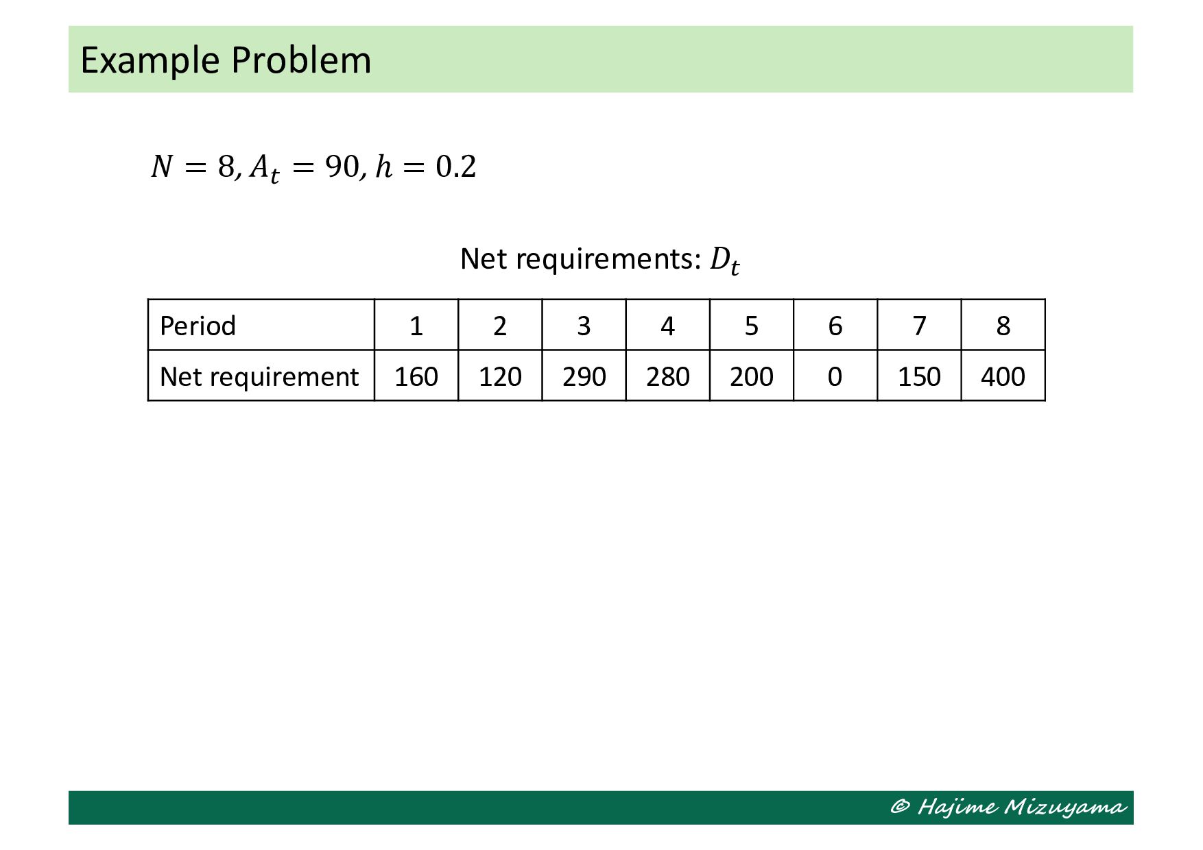
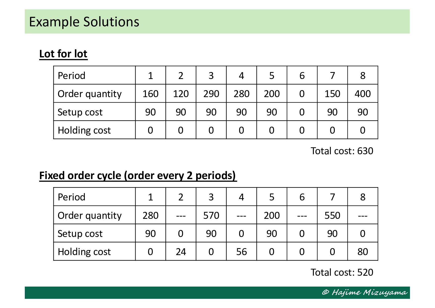
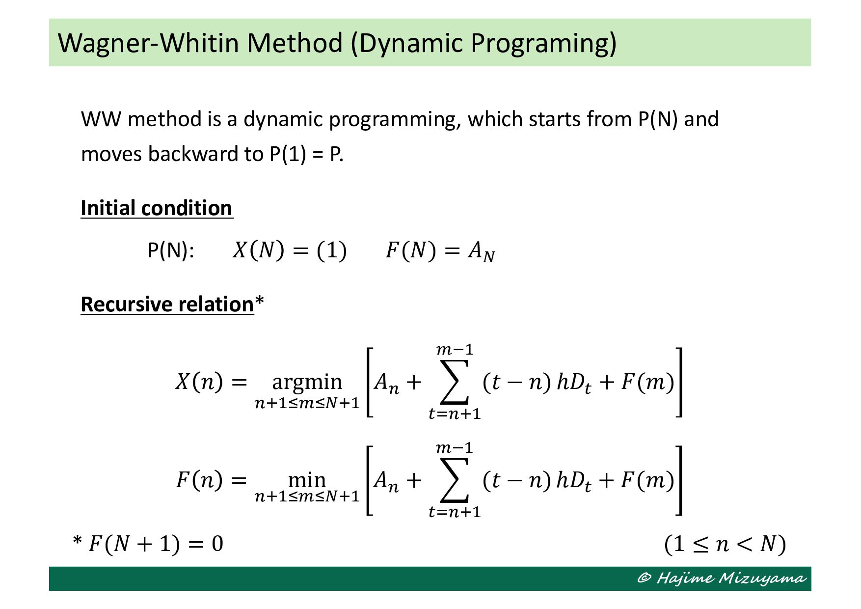
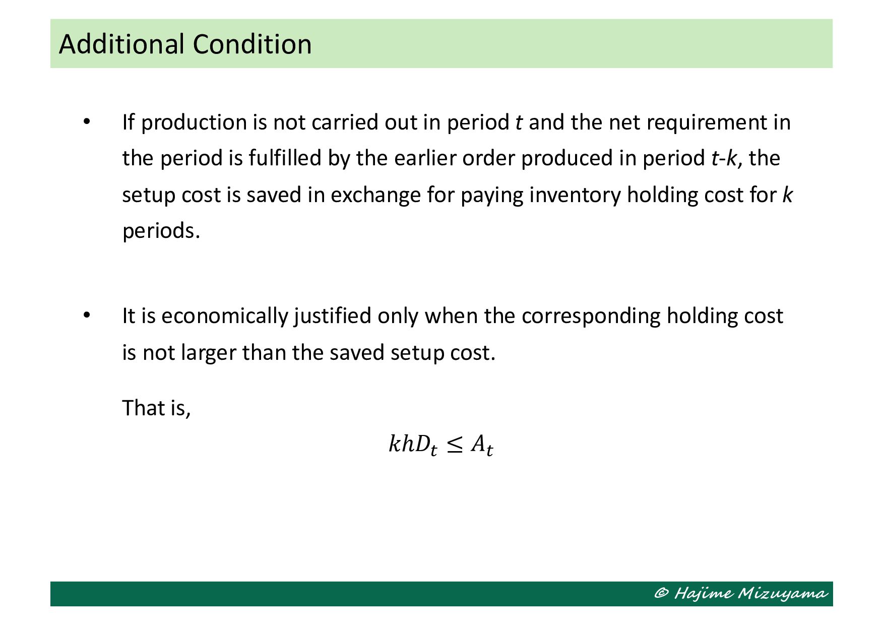
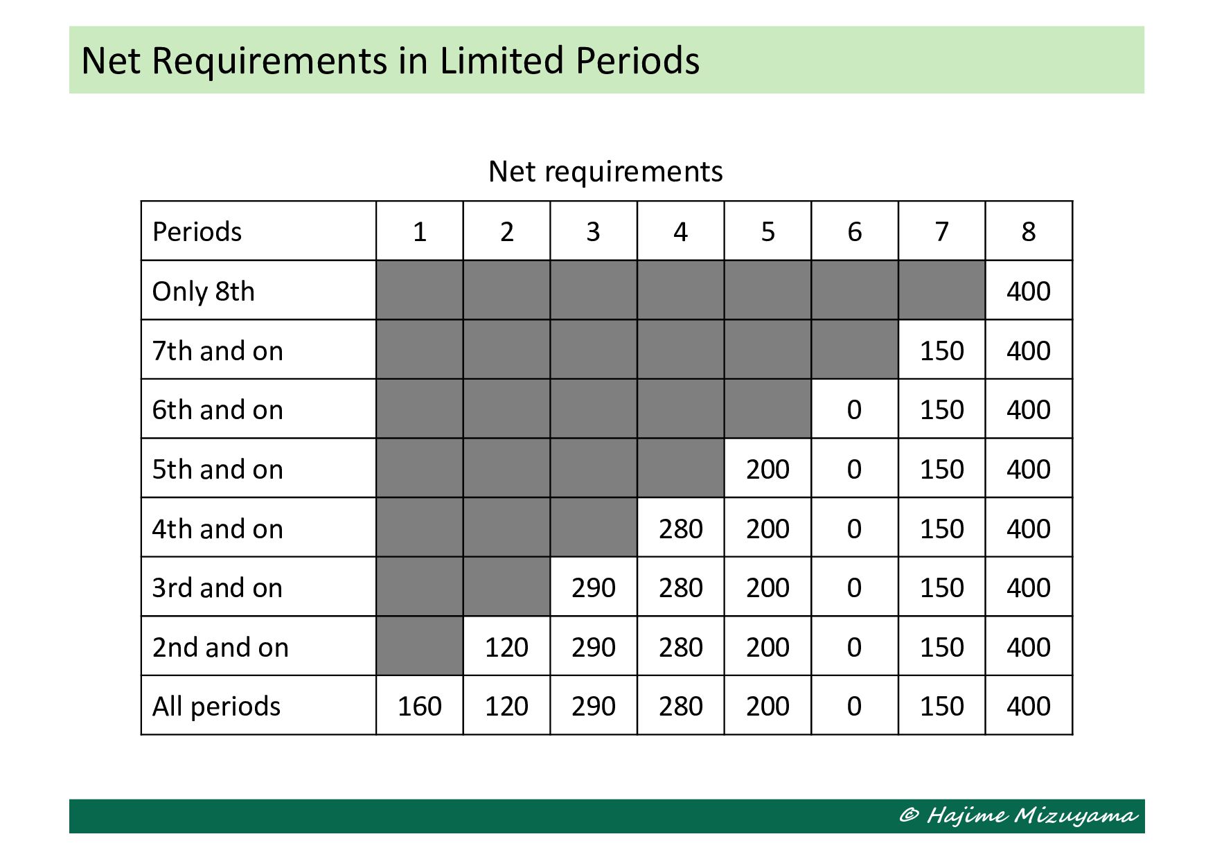
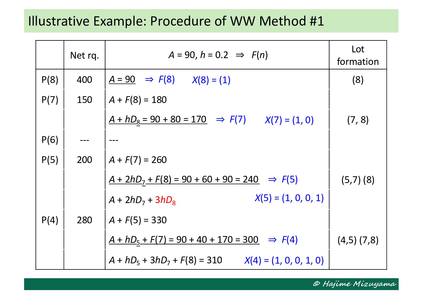
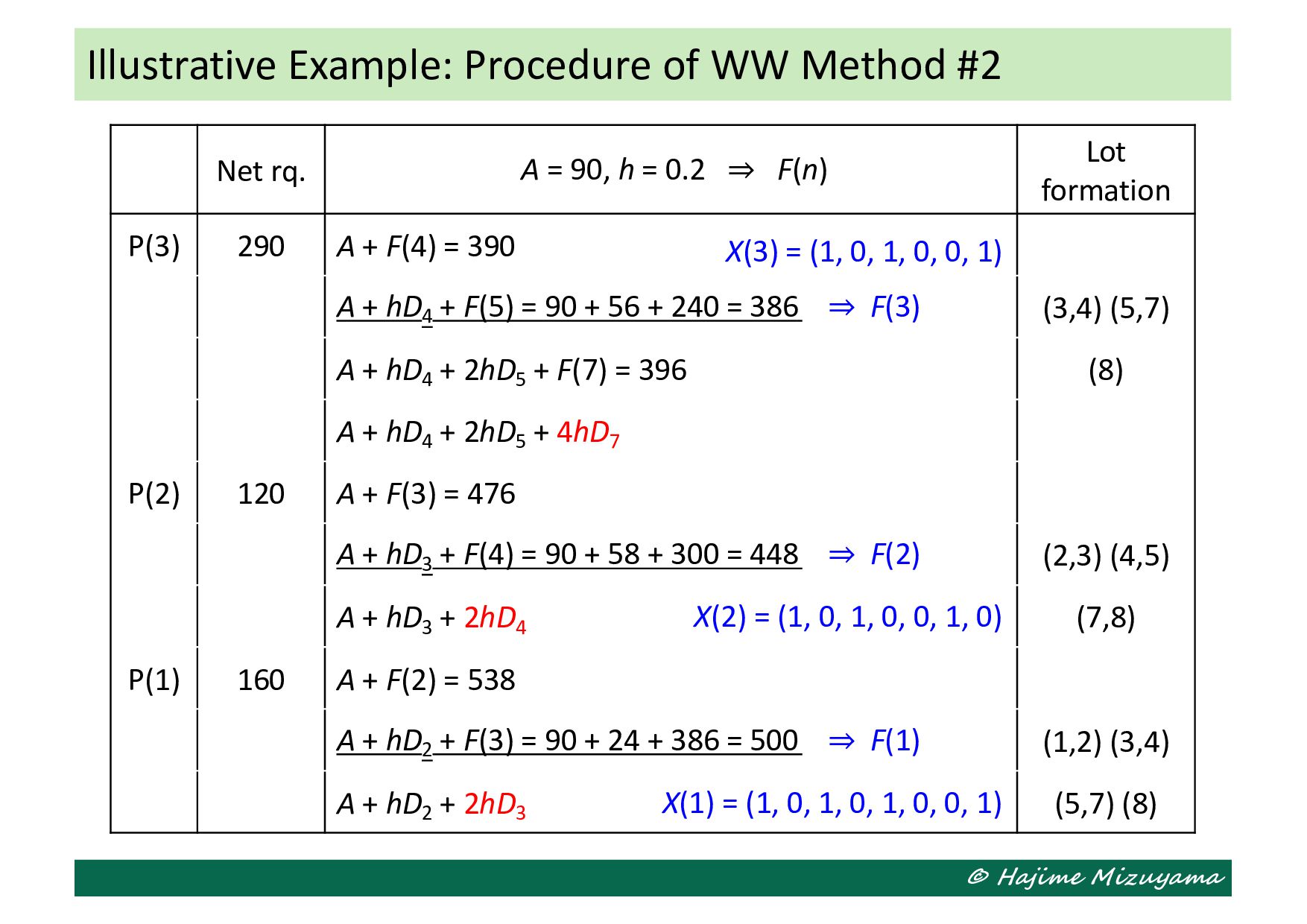
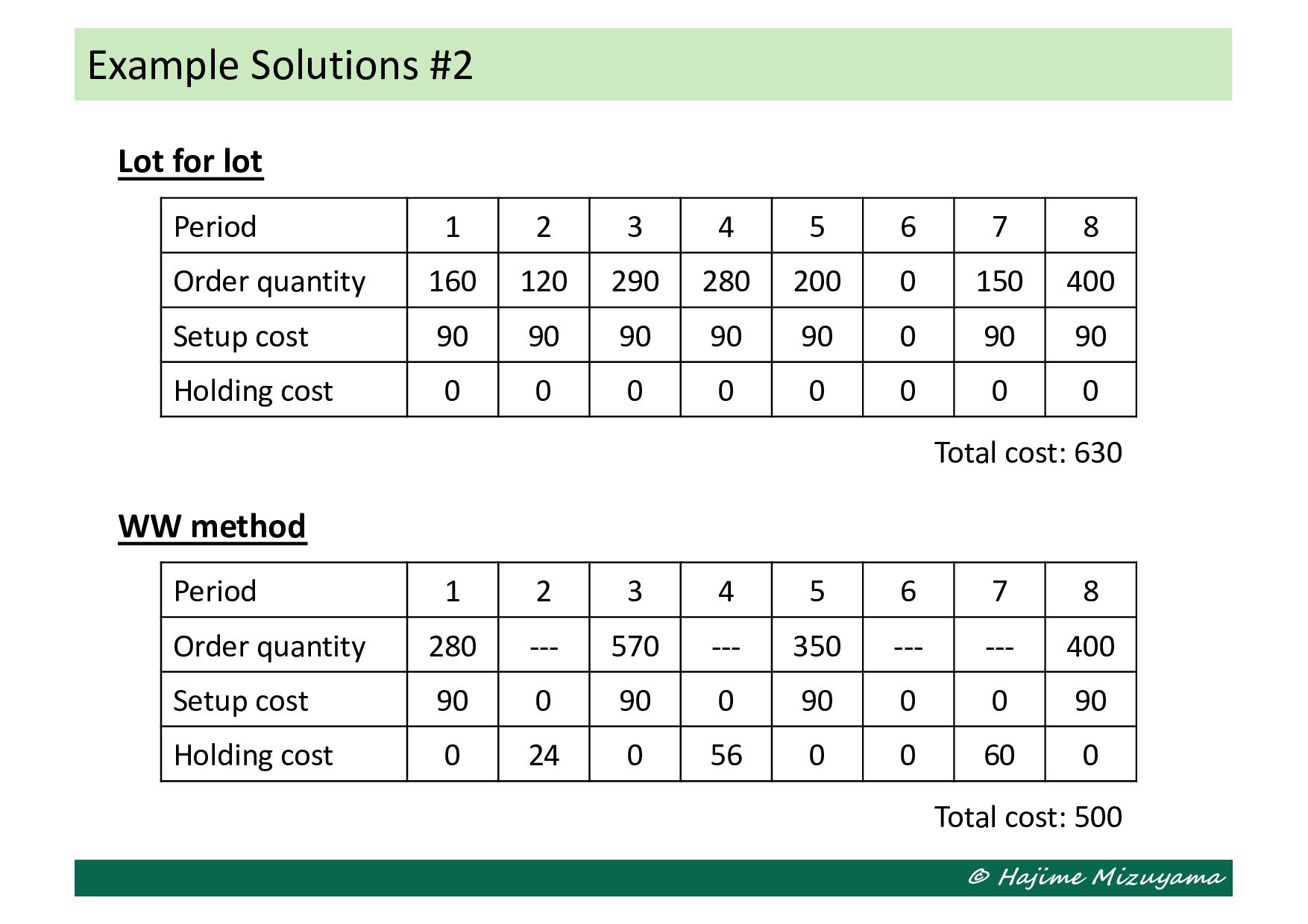
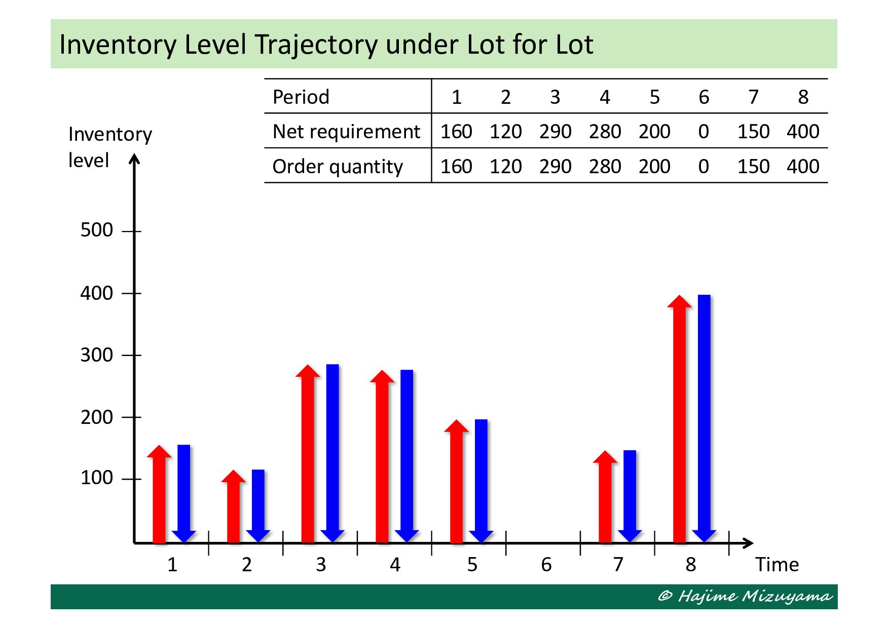
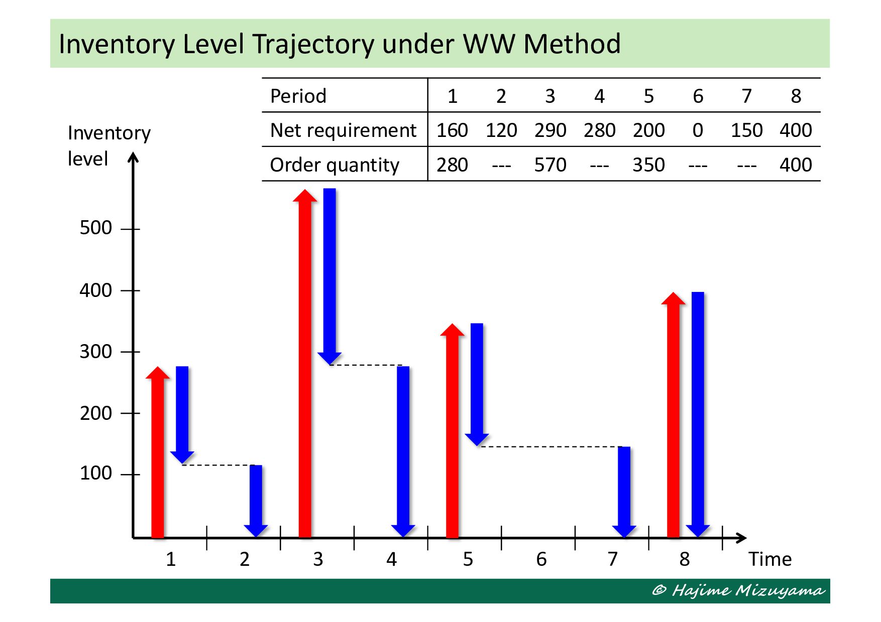
13. © Hajime Mizuyama Net rq. A = 90, h = 0.2 ⇒ F(n) Lot formation P(3) 290 A + F(4) = 390 A + hD4 + F(5) = 90 + 56 + 240 = 386 ⇒ F(3) (3,4) (5,7) A + hD4 + 2hD5 + F(7) = 396 (8) A + hD4 + 2hD5 + 4hD7 P(2) 120 A + F(3) = 476 A + hD3 + F(4) = 90 + 58 + 300 = 448 ⇒ F(2) (2,3) (4,5) A + hD3 + 2hD4 (7,8) P(1) 160 A + F(2) = 538 A + hD2 + F(3) = 90 + 24 + 386 = 500 ⇒ F(1) (1,2) (3,4) A + hD2 + 2hD3 (5,7) (8) Illustrative Example: Procedure of WW Method #2 X(3) = (1, 0, 1, 0, 0, 1) X(2) = (1, 0, 1, 0, 0, 1, 0) X(1) = (1, 0, 1, 0, 1, 0, 0, 1)
14. © Hajime Mizuyama Period 1 2 3 4 5 6 7 8 Order quantity 160 120 290 280 200 0 150 400 Setup cost 90 90 90 90 90 0 90 90 Holding cost 0 0 0 0 0 0 0 0 Example Solutions #2 Total cost: 630 Lot for lot Period 1 2 3 4 5 6 7 8 Order quantity 280 --- 570 --- 350 --- --- 400 Setup cost 90 0 90 0 90 0 0 90 Holding cost 0 24 0 56 0 0 60 0 Total cost: 500 WW method
15. © Hajime Mizuyama Period 1 2 3 4 5 6 7 8 Net requirement 160 120 290 280 200 0 150 400 Order quantity 160 120 290 280 200 0 150 400 Inventory Level Trajectory under Lot for Lot Time 100 200 300 400 1 2 3 4 5 6 7 Inventory level 8 500
16. © Hajime Mizuyama Inventory Level Trajectory under Fixed Order Cycle Time 100 200 300 400 1 2 3 4 5 6 7 Inventory level Period 1 2 3 4 5 6 7 8 Net requirement 160 120 290 280 200 0 150 400 Order quantity 280 --- 570 --- 200 --- 550 --- 8 500
17. © Hajime Mizuyama Inventory Level Trajectory under WW Method Time 100 200 300 400 1 2 3 4 5 6 7 Inventory level Period 1 2 3 4 5 6 7 8 Net requirement 160 120 290 280 200 0 150 400 Order quantity 280 --- 570 --- 350 --- --- 400 8 500