Introduction of Mask R-CNN

Transcript

1. Mask R-CNNによる 物体検出とセグメンテーションの マルチタスク学習 板垣 正敏 2019/8/24 @Python機械学習勉強会in新潟 Restart#8
2. 主な画像系深層学習タスク （⽣成系を除く）
3. 画像認識 š画像全体を⼊⼒として、何が 写っているかをラベル付け šディープニューラルネット ワーク、特に畳み込みニュー ラルネットワークのパワーを 最初に⾒せつけた分野 Figure 4: (Left) Eight ILSVRC-2010 test images and the five The correct label is written under each image, and the probab with a red bar (if it happens to be in the top 5). (Right) Five IL https://papers.nips.cc/paper/4824-imagenet-classification-with-deep-convolutional-neural-networks.pdf
4. 基本となるのは CNN（畳み込みニューラルネットワーク） 150x150x3 148x148x32 74x74x32 72x72x64 36x36x64 34x34x128 17x17x128 15x15x128 7x7x128 6272 512 1 conv3x3, 32 stride (1, 1) maxpool2x2 stride (2, 2) conv3x3, 64 stride (1, 1) maxpool2x2 stride (2, 2) conv3x3, 128 stride (1, 1) maxpool2x2 stride (2, 2) conv3x3, 128 stride (1, 1) maxpool2x2 stride (2, 2) flatten flatten dense dense dense dense ・ （積和） カーネル （フィルタ）
5. 物体検出 š画像の中に存在す る物体の位置（四 ⾓形であることが 多い）と物体の種 別を判別 https://arxiv.org/abs/1506.01497
6. セグメンテーション š画像のピクセル単位でそのピ クセルがなんの物体に属して いるかを判別 š⾔い換えれば、物体の塗りつ ぶしあるいはマスキング http://jamie.shotton.org/work/research.html
7. 物体検出モデルの系譜
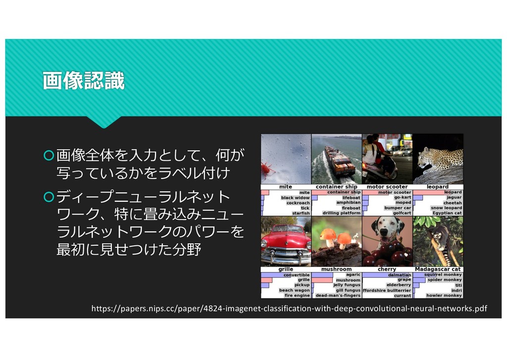
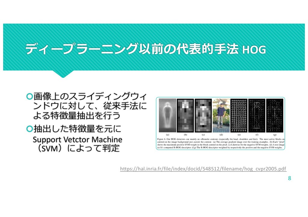
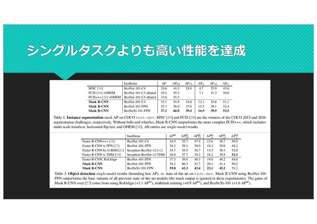
8. ディープラーニング以前の代表的⼿法 HOG š画像上のスライディングウィ ンドウに対して、従来⼿法に よる特徴量抽出を⾏う š抽出した特徴量を元に Support Vetctor Machine （SVM）によって判定 (a) (b) (c) (d) (e) (f) (g) Figure 6. Our HOG detectors cue mainly on silhouette contours (especially the head, shoulders and feet). The most active blocks are centred on the image background just outside the contour. (a) The average gradient image over the training examples. (b) Each “pixel” shows the maximum positive SVM weight in the block centred on the pixel. (c) Likewise for the negative SVM weights. (d) A test image. (e) It’s computed R-HOG descriptor. (f,g) The R-HOG descriptor weighted by respectively the positive and the negative SVM weights. would help to improve the detection results in more general situations. Acknowledgments. This work was supported by the Euro- pean Union research projects ACEMEDIA and PASCAL. We thanks Cordelia Schmid for many useful comments. SVM- Light [10] provided reliable training of large-scale SVM’s. References [1] S. Belongie, J. Malik, and J. Puzicha. Matching shapes. The 8th ICCV, Vancouver, Canada, pages 454–461, 2001. [2] V. de Poortere, J. Cant, B. Van den Bosch, J. de Prins, F. Fransens, and L. Van Gool. Efficient pedes- trian detection: a test case for svm based categorization. Workshop on Cognitive Vision, 2002. Available online: http://www.vision.ethz.ch/cogvis02/. [3] P. Felzenszwalb and D. Huttenlocher. Efficient matching of pictorial structures. CVPR, Hilton Head Island, South Car- olina, USA, pages 66–75, 2000. [4] W. T. Freeman and M. Roth. Orientation histograms for hand gesture recognition. Intl. Workshop on Automatic Face- and Gesture- Recognition, IEEE Computer Society, Zurich, [10] T. Joachims. Making large-scale svm learning practical. In B. Schlkopf, C. Burges, and A. Smola, editors, Advances in Kernel Methods - Support Vector Learning. The MIT Press, Cambridge, MA, USA, 1999. [11] Y. Ke and R. Sukthankar. Pca-sift: A more distinctive rep- resentation for local image descriptors. CVPR, Washington, DC, USA, pages 66–75, 2004. [12] D. G. Lowe. Distinctive image features from scale-invariant keypoints. IJCV, 60(2):91–110, 2004. [13] R. K. McConnell. Method of and apparatus for pattern recog- nition, January 1986. U.S. Patent No. 4,567,610. [14] K. Mikolajczyk and C. Schmid. A performance evaluation of local descriptors. PAMI, 2004. Accepted. [15] K. Mikolajczyk and C. Schmid. Scale and affine invariant interest point detectors. IJCV, 60(1):63–86, 2004. [16] K. Mikolajczyk, C. Schmid, and A. Zisserman. Human detec- tion based on a probabilistic assembly of robust part detectors. The 8th ECCV, Prague, Czech Republic, volume I, pages 69– 81, 2004. [17] A. Mohan, C. Papageorgiou, and T. Poggio. Example-based 8 https://hal.inria.fr/file/index/docid/548512/filename/hog_cvpr2005.pdf
9. R-CNN (Region-based CNN) š HOGの特徴検出器の代わりにCNNを使う š スライディング・ウィンドウでしらみつぶしにCNNによる判定を⾏うのは ⾮現実的 š 物体らしさ(Objectness)を⾒つける既存⼿法(Selective Search)を⽤いて、画 像から領域候補(Region Proposals)を探す(2000個程度) š 領域候補の領域画像を 全て⼀定の⼤きさにリサイズして CNNにかけて特 徴量を取り出す š 取り出した特徴量を使って複数のSVMによって学習しカテゴリ識別、 regressorによってBounding Box の正確な位置を推定 https://arxiv.org/abs/1311.2524
10. IoUとNMS š IoU: Intersection over Union š領域の重なり具合の評価指標 š NMS: Non-Maximum Suppression š1つの正解（Ground Truth）に対す る複数の領域候補の重なり具合を IoU で評価し、IoU が最⼤のもの だけを残して他を捨てることで、 計算量を抑制する⼿法 https://qiita.com/mshinoda88/items/9770ee671ea27f2c81a9
11. SPP-net (spatial pyramid pooling) š R-CNNでは、2000の領域候補を 同じサイズの画像に変形したの ち、全てCNNにかけて特徴抽出 をしているため、計算量が多い š SPPでは、CNNによって画像全体 の特徴マップを⽣成し、この特 徴マップに階層的プーリングを ⾏うことで、任意のサイズの⼊ ⼒画像を扱えるようにしながら、 計算量を抑制する https://arxiv.org/abs/1406.4729
12. Fast R-CNN šRoI pooling layerという、SPPのpyramid構造を取り除いたシンプ ルな幅可変poolingを⾏う šclassification/bounding box regressionを同時に学習させるため の multi-task loss によって1回で学習ができるようにする šVGG16を⽤いたR-CNNより9倍の学習速度、213倍の識別速度 š SPPnetの3倍の学習速度、10倍の識別速度 https://arxiv.org/abs/1504.08083
13. RoI(Region of Intrest) Pooling š 単純で効率的なプーリング⼿法 š 領域候補を同じサイズのセクショ ンに分割（その数は出⼒の次元と 同じ） š 各セクションで最⼤値を⾒つける š これらの最⼤値を出⼒バッファに コピーする https://qiita.com/mshinoda88/items/9770ee671ea27f2c81a9
14. Faster R-CNN š RPN(Region Proposal Network) の導⼊とEnd- to-End 学習 š アンカーボックスを出 発点に物体の存在しそ うな領域を推定するサ ブネットワークを提案 https://arxiv.org/abs/1506.01497
15. RPN Anchor Boxを出発点に 物体のありそうな領域 を抽出 Region Proposal Network • 特徴マップ上にAnchorを定義（方眼紙に見立てて、各マスの中心のイメージ） • 各Anchor毎にk個のAnchor Boxを定義（スケールとアスペクト比の組み合わせ） • 各Anchor Box毎に、物体らしさのスコアと位置・サイズの修正項を予測するように訓練する Faster R-CNN: http://arxiv.org/abs/1506.01497 画像 特徴 マップ CNN (特徴抽出） ・・・ スケール アスペクト比 × 各アンカーごとにk個のBox （例: k = 3 × 3） 2k scores （物体 or 背景） 4k coordinates （x, y, w, hの 修正項） H x W x 3 H/16 x W/16 x 3 8 https://www.slideshare.net/ToshinoriHanya/ohs3
16. YOLO š領域をあらかじめ決めたグ リッドに分割 šグリッド単位の物体の存在可 能性と、領域の位置・サイズ を推定 https://www.cv-foundation.org/openaccess/content_cvpr_2016/papers/Redmon_You_Only_Look_CVPR_2016_paper.pdf
17. FPN (Feature Pyramid Net) š さまざまなスケールの物体を検出するた めの⼯夫 š CNNの各層の出⼒を特徴として取り出す ボトムアップ処理 š 低解像度で意味的にはっきりした特徴 マップをアップサンプリングし、より⾼ 解像度の特徴マップと混合することでよ り解像度の⾼い検出を⾏うボトムアップ 処理 https://arxiv.org/abs/1612.03144
18. YOLO v.2 šFaster R-CNNなどのアイデアを取り込み性能アップ šBachNormalizationの導⼊ š⾼解像度化 šAnchor Boxの導⼊ šIoUに基づく距離を使ったk-means法によるBouding Boxのクラス タリング šBox位置の直接推定 https://pjreddie.com/darknet/yolov2/
19. SSD CNNの各層の特徴 マップを使って領 域と物体を同時に 推定 https://arxiv.org/abs/1512.02325
20. RetinaNet š Facebook AI Researchに よる提案 š 分類器にFocal Lossを導 ⼊（前景後景のオブ ジェクトの不均衡分類 対策） š ResNetの複数の層の特 徴マップを使い、クラ ス分類器とBox推定器 を訓練 class+box subnets class subnet box subnet W×H ×256 W×H ×256 W×H ×4A W×H ×256 W×H ×256 W×H ×KA ×4 ×4 + + class+box subnets class+box subnets (a) ResNet (b) feature pyramid net (c) class subnet (top) (d) box subnet (bottom) Figure 3. The one-stage RetinaNet network architecture uses a Feature Pyramid Network (FPN) [20] backbone on top of a feedforward ResNet architecture [16] (a) to generate a rich, multi-scale convolutional feature pyramid (b). To this backbone RetinaNet attaches two subnetworks, one for classifying anchor boxes (c) and one for regressing from anchor boxes to ground-truth object boxes (d). The network design is intentionally simple, which enables this work to focus on a novel focal loss function that eliminates the accuracy gap between our one-stage detector and state-of-the-art two-stage detectors like Faster R-CNN with FPN [20] while running at faster speeds. Classification Subnet: The classification subnet predicts the probability of object presence at each spatial position for each of the A anchors and K object classes. This subnet is a small FCN attached to each FPN level; parameters of this subnet are shared across all pyramid levels. Its design is simple. Taking an input feature map with C channels from a given pyramid level, the subnet applies four 3⇥3 conv layers, each with C filters and each followed by ReLU activations, followed by a 3⇥3 conv layer with KA filters. Finally sigmoid activations are attached to output the KA binary predictions per spatial location, see Figure 3 (c). We use C = 256 and A = 9 in most experiments. In contrast to RPN [28], our object classification subnet is deeper, uses only 3⇥3 convs, and does not share param- eters with the box regression subnet (described next). We found these higher-level design decisions to be more im- portant than specific values of hyperparameters. Box Regression Subnet: In parallel with the object classi- fication subnet, we attach another small FCN to each pyra- mid level for the purpose of regressing the offset from each anchor box to a nearby ground-truth object, if one exists. The design of the box regression subnet is identical to the classification subnet except that it terminates in 4A linear regression subnet, see Figure 3. As such, inference involves simply forwarding an image through the network. To im- prove speed, we only decode box predictions from at most 1k top-scoring predictions per FPN level, after threshold- ing detector confidence at 0.05. The top predictions from all levels are merged and non-maximum suppression with a threshold of 0.5 is applied to yield the final detections. Focal Loss: We use the focal loss introduced in this work as the loss on the output of the classification subnet. As we will show in §5, we find that = 2 works well in practice and the RetinaNet is relatively robust to 2 [0.5, 5]. We emphasize that when training RetinaNet, the focal loss is applied to all ⇠100k anchors in each sampled image. This stands in contrast to common practice of using heuristic sampling (RPN) or hard example mining (OHEM, SSD) to select a small set of anchors (e.g., 256) for each minibatch. The total focal loss of an image is computed as the sum of the focal loss over all ⇠100k anchors, normalized by the number of anchors assigned to a ground-truth box. We per- form the normalization by the number of assigned anchors, not total anchors, since the vast majority of anchors are easy negatives and receive negligible loss values under the focal loss. Finally we note that ↵, the weight assigned to the rare https://arxiv.org/abs/1708.02002
21. YOLO v3 š Bounding Boxの指標に誤差⾃乗和を採⽤ š 物体らしさの評価にロジスティック回 帰を使⽤ š クラス分類にSoftmaxではなくロジス ティック回帰によるマルチラベル識別 器を使⽤ š マルチスケールなBounding Box予測 š ⾼速化のため新しい特徴抽出ネット ワークを使⽤ YOLOv3: An Incremental Improvement Joseph Redmon, Ali Farhadi University of Washington Abstract We present some updates to YOLO! We made a bunch of little design changes to make it better. We also trained this new network that’s pretty swell. It’s a little bigger than last time but more accurate. It’s still fast though, don’t worry. At 320 ⇥ 320 YOLOv3 runs in 22 ms at 28.2 mAP, as accurate as SSD but three times faster. When we look at the old .5 IOU mAP detection metric YOLOv3 is quite good. It achieves 57.9 AP50 in 51 ms on a Titan X, com- pared to 57.5 AP50 in 198 ms by RetinaNet, similar perfor- mance but 3.8⇥ faster. As always, all the code is online at https://pjreddie.com/yolo/. 1. Introduction Sometimes you just kinda phone it in for a year, you know? I didn’t do a whole lot of research this year. Spent a lot of time on Twitter. Played around with GANs a little. I had a little momentum left over from last year [12] [1]; I managed to make some improvements to YOLO. But, hon- estly, nothing like super interesting, just a bunch of small changes that make it better. I also helped out with other people’s research a little. Actually, that’s what brings us here today. We have a camera-ready deadline [4] and we need to cite some of the random updates I made to YOLO but we don’t have a source. So get ready for a TECH REPORT! The great thing about tech reports is that they don’t need intros, y’all know why we’re here. So the end of this intro- duction will signpost for the rest of the paper. First we’ll tell you what the deal is with YOLOv3. Then we’ll tell you how 50 100 150 200 250 inference time (ms) 28 30 32 34 36 38 COCO AP B C D E F G RetinaNet-50 RetinaNet-101 YOLOv3 Method [B] SSD321 [C] DSSD321 [D] R-FCN [E] SSD513 [F] DSSD513 [G] FPN FRCN RetinaNet-50-500 RetinaNet-101-500 RetinaNet-101-800 YOLOv3-320 YOLOv3-416 YOLOv3-608 mAP 28.0 28.0 29.9 31.2 33.2 36.2 32.5 34.4 37.8 28.2 31.0 33.0 time 61 85 85 125 156 172 73 90 198 22 29 51 Figure 1. We adapt this figure from the Focal Loss paper [9]. YOLOv3 runs significantly faster than other detection methods with comparable performance. Times from either an M40 or Titan X, they are basically the same GPU. 2.1. Bounding Box Prediction Following YOLO9000 our system predicts bounding boxes using dimension clusters as anchor boxes [15]. The network predicts 4 coordinates for each bounding box, tx , ty , tw , th . If the cell is offset from the top left corner of the image by (cx, cy) and the bounding box prior has width and height pw , ph , then the predictions correspond to: bx = (tx) + cx by = (ty) + cy bw = pwetw bh = pheth https://arxiv.org/abs/1804.02767
22. Mask R-CNNとその実装例
23. Mask R-CNN ≒ Faster R-CNN + Mask Branch https://arxiv.org/abs/1703.06870
24. シングルタスクよりも⾼い性能を達成 backbone APbb APbb 50 APbb 75 APbb S APbb M APbb L Faster R-CNN+++ [19] ResNet-101-C4 34.9 55.7 37.4 15.6 38.7 50.9 Faster R-CNN w FPN [27] ResNet-101-FPN 36.2 59.1 39.0 18.2 39.0 48.2 Faster R-CNN by G-RMI [21] Inception-ResNet-v2 [41] 34.7 55.5 36.7 13.5 38.1 52.0 Faster R-CNN w TDM [39] Inception-ResNet-v2-TDM 36.8 57.7 39.2 16.2 39.8 52.1 Faster R-CNN, RoIAlign ResNet-101-FPN 37.3 59.6 40.3 19.8 40.2 48.8 Mask R-CNN ResNet-101-FPN 38.2 60.3 41.7 20.1 41.1 50.2 Mask R-CNN ResNeXt-101-FPN 39.8 62.3 43.4 22.1 43.2 51.2 Table 3. Object detection single-model results (bounding box AP), vs. state-of-the-art on test-dev. Mask R-CNN using ResNet-101- FPN outperforms the base variants of all previous state-of-the-art models (the mask output is ignored in these experiments). The gains of Mask R-CNN over [27] come from using RoIAlign (+1.1 APbb), multitask training (+0.9 APbb), and ResNeXt-101 (+1.6 APbb). (50% relative improvement). Moreover, we note that with RoIAlign, using stride-32 C5 features (30.9 AP) is more ac- curate than using stride-16 C4 features (30.3 AP, Table 2c). RoIAlign largely resolves the long-standing challenge of using large-stride features for detection and segmentation. Finally, RoIAlign shows a gain of 1.5 mask AP and 0.5 4.4. Timing Inference: We train a ResNet-101-FPN model that shares features between the RPN and Mask R-CNN stages, follow- ing the 4-step training of Faster R-CNN [36]. This model runs at 195ms per image on an Nvidia Tesla M40 GPU (plus 15ms CPU time resizing the outputs to the original resolu- Figure 5. More results of Mask R-CNN on COCO test images, using ResNet-101-FPN and running at 5 fps, with 35.7 mask AP (Table 1). backbone AP AP50 AP75 APS APM APL MNC [10] ResNet-101-C4 24.6 44.3 24.8 4.7 25.9 43.6 FCIS [26] +OHEM ResNet-101-C5-dilated 29.2 49.5 - 7.1 31.3 50.0 FCIS+++ [26] +OHEM ResNet-101-C5-dilated 33.6 54.5 - - - - Mask R-CNN ResNet-101-C4 33.1 54.9 34.8 12.1 35.6 51.1 Mask R-CNN ResNet-101-FPN 35.7 58.0 37.8 15.5 38.1 52.4 Mask R-CNN ResNeXt-101-FPN 37.1 60.0 39.4 16.9 39.9 53.5 Table 1. Instance segmentation mask AP on COCO test-dev. MNC [10] and FCIS [26] are the winners of the COCO 2015 and 2016 segmentation challenges, respectively. Without bells and whistles, Mask R-CNN outperforms the more complex FCIS+++, which includes multi-scale train/test, horizontal flip test, and OHEM [38]. All entries are single-model results. can predict K masks per RoI, but we only use the k-th mask, where k is the predicted class by the classification branch. The m⇥m floating-number mask output is then resized to the RoI size, and binarized at a threshold of 0.5. Note that since we only compute masks on the top 100 detection boxes, Mask R-CNN adds a small overhead to its Faster R-CNN counterpart (e.g., ⇠20% on typical models). 4. Experiments: Instance Segmentation We perform a thorough comparison of Mask R-CNN to the state of the art along with comprehensive ablations on the COCO dataset [28]. We report the standard COCO met- rics including AP (averaged over IoU thresholds), AP50 , AP75 , and APS , APM , APL (AP at different scales). Un- less noted, AP is evaluating using mask IoU. As in previous work [5, 27], we train using the union of 80k train images and a 35k subset of val images (trainval35k), and re- 4.1. Main Results We compare Mask R-CNN to the state-of-the-art meth- ods in instance segmentation in Table 1. All instantia- tions of our model outperform baseline variants of pre- vious state-of-the-art models. This includes MNC [10] and FCIS [26], the winners of the COCO 2015 and 2016 segmentation challenges, respectively. Without bells and whistles, Mask R-CNN with ResNet-101-FPN backbone outperforms FCIS+++ [26], which includes multi-scale train/test, horizontal flip test, and online hard example min- ing (OHEM) [38]. While outside the scope of this work, we expect many such improvements to be applicable to ours. Mask R-CNN outputs are visualized in Figures 2 and 5. Mask R-CNN achieves good results even under challeng- ing conditions. In Figure 6 we compare our Mask R-CNN baseline and FCIS+++ [26]. FCIS+++ exhibits systematic artifacts on overlapping instances, suggesting that it is chal-
25. https://github.com/matterport/Mask_RCNN
26. さまざまな実装例 šmatterport/Mask_RCNN šKeras による実装 š tensorflow/models šTensorFlow Object Detection API の機能として実装 šfacebookresearch/detectron šFacebook の Object Detection System の⼀部として実装（Caffe2ベース） š facebookresearch/maskrcnn-benchmark šPyTorch による実装
27. 訓練⽤データセット šPASCAL VOC šhttp://host.robots.ox.ac.uk/pascal/VOC/ š2005年から2012年まで⾏われたコンテストのデータセット šMS COCO šhttp://cocodataset.org/ šMicrosoftが提供しているデータセット š2014年、2015年、2017年のデータセット š2018年、2019年にはキーポイント検出や姿勢推定のアノテーションも 追加
28. カスタムトレーニングと留意事項 šデータセットやモデルによって訓練⽤データセットのアノテー ションの形式が異なる šXML、JSON、CSVなど š物体検出の位置情報も、左上、右下の座標を前提とするものと、 中⼼の座標と⾼さと幅を前提とするものがある šマスクのアノテーションも、ビットマップ（バイナリ、整数） や、RLEによって圧縮されたものなどさまざま
29. アノテーションツール šCVAT (Computer Vision Annotation Tool) šhttps://github.com/opencv/cvat šOpenCV が提供している画像アノンテーションツール š画像分類、物体検出、セグメンテーションに対応 šDockerを使って起動可能 šAbeja Platform Annotation （有料サービス） šhttps://abejainc.com/platform/ja/
30. コンテスト š SIIM-ACR Pneumothorax Segmentation -- Identify Pneumothorax disease in chest x-rays šhttps://www.kaggle.com/c/siim-acr-pneumothorax-segmentation šレントゲン画像から気胸の部位を検出する šもうすぐコンペ終了 š 2018 Data Science Bowl -- Find the nuclei in divergent images to advance medical discovery šhttps://www.kaggle.com/c/data-science-bowl-2018 š顕微鏡写真から細胞核を検出する š終了したコンペ
31. まとめ
32. Mask R-CNNの使い所 š Mask R-CNNは、物体検出とセグメンテーション、キーポイント検出を同 時に⾏えるモデル š 物体検出だけ、セグメンテーションだけを⾏うモデルよりも⾼い精度が 期待できる š 画像診断や故障部位検出などの分野に応⽤可能と考えられる š ベースとなるCNNや物体検出やセグメンテーションのデータセットで訓練 済みのネットワークを使い、転移学習・ファインチューニングが可能 š ただし、物体検出の推論スピードは、YOLOやSSDなどに⽐べて速くないの で、⽬的によっては留意が必要
33. 参考
34. 参考にした記事等 š 物体検出、セグメンテーションをMask R-CNNで理解してみる (初⼼者) š https://qiita.com/shtamura/items/4283c851bc3d9721ed96 š 物体検出についての歴史まとめ š https://qiita.com/mshinoda88/items/9770ee671ea27f2c81a9 š 物体検出モデルの進展 Part3 ~FPNとRetinaNet~ š https://qiita.com/TaigaHasegawa/items/653abc81ac4ee1f0d7b8 š アノテーションツール(正解⼊⼒ツール)が進化している。 2 š https://qiita.com/nonbiri15/items/819efb0d42b1541c29c0 š 画像を扱う機械学習のためのデータセットまとめ š https://qiita.com/leetmikeal/items/7c0d23e39bf38ab8be23