QGP parameter extraction via a global analysis of event-by-event flow coefficient distributions

Prelim exam talk at Duke.

Transcript

1. QGP parameter extraction via a global analysis of event-by-event flow coefficient distributions Jonah Bernhard Preliminary exam January 6, 2014
2. Model-to-data comparison Data Computer model Inferences Predictions 1 / 29
3. Model-to-data comparison: heavy-ion collisions Model Initial conditions, τ0, η/s, . . . 0.00 0.05 0.10 0.15 0.20 v2 0 5 10 15 20 P(v2 ) thick black line = ATLAS thin colored lines = model glb v2 20 25% 2 / 29
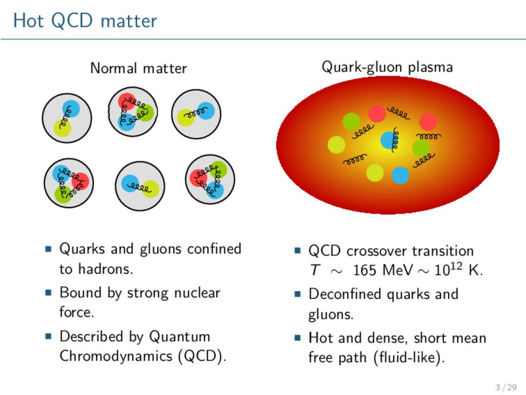
4. Hot QCD matter Normal matter Quarks and gluons confined to hadrons. Bound by strong nuclear force. Described by Quantum Chromodynamics (QCD). Quark-gluon plasma QCD crossover transition T ∼ 165 MeV ∼ 1012 K. Deconfined quarks and gluons. Hot and dense, short mean free path (fluid-like). 3 / 29
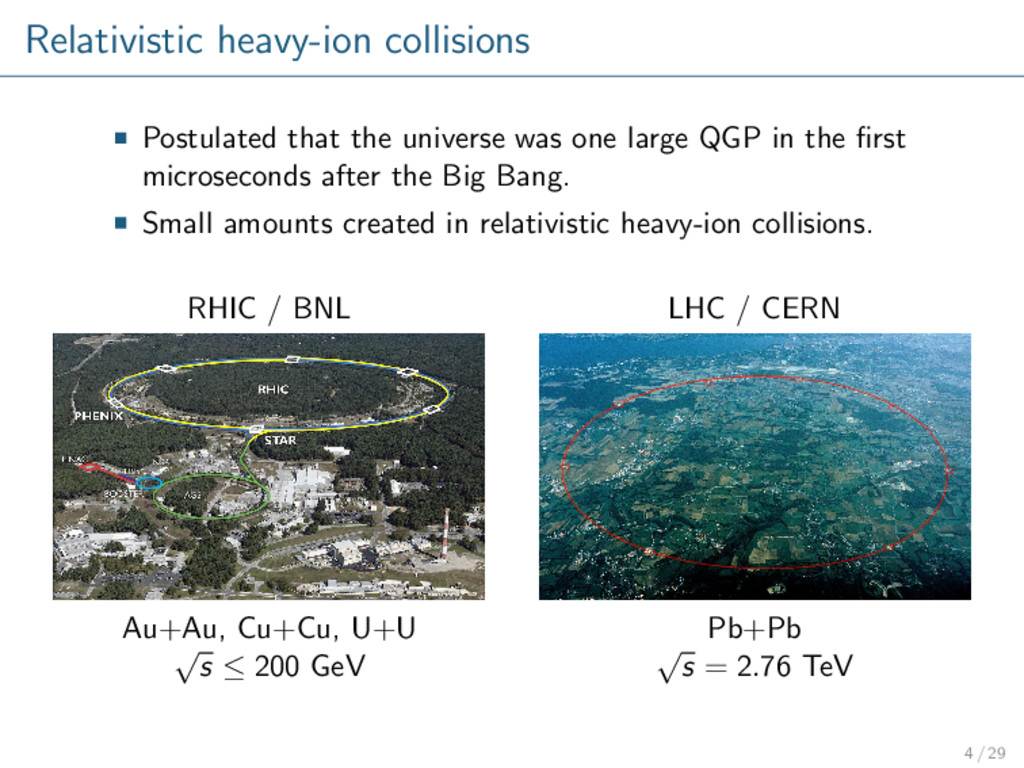
5. Relativistic heavy-ion collisions Postulated that the universe was one large QGP in the first microseconds after the Big Bang. Small amounts created in relativistic heavy-ion collisions. RHIC / BNL Au+Au, Cu+Cu, U+U √ s ≤ 200 GeV LHC / CERN Pb+Pb √ s = 2.76 TeV 4 / 29
6. Spacetime evolution x ∼ 10−14 m t ∼ 10−23 s z t Hot and dense QGP, Hydrodynamic expansion Pre-equilibrium Thermalization Freeze-out Hadron gas Proper time 5 / 29
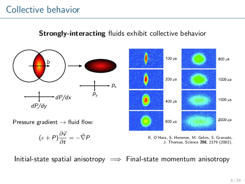
7. Collective behavior Strongly-interacting fluids exhibit collective behavior dP/dx dP/dy p x p y b Pressure gradient → fluid flow: ( + P) ∂v ∂t = −∇P K. O’Hara, S. Hemmer, M. Gehm, S. Granade, J. Thomas, Science 298, 2179 (2002). Initial-state spatial anisotropy =⇒ Final-state momentum anisotropy 6 / 29
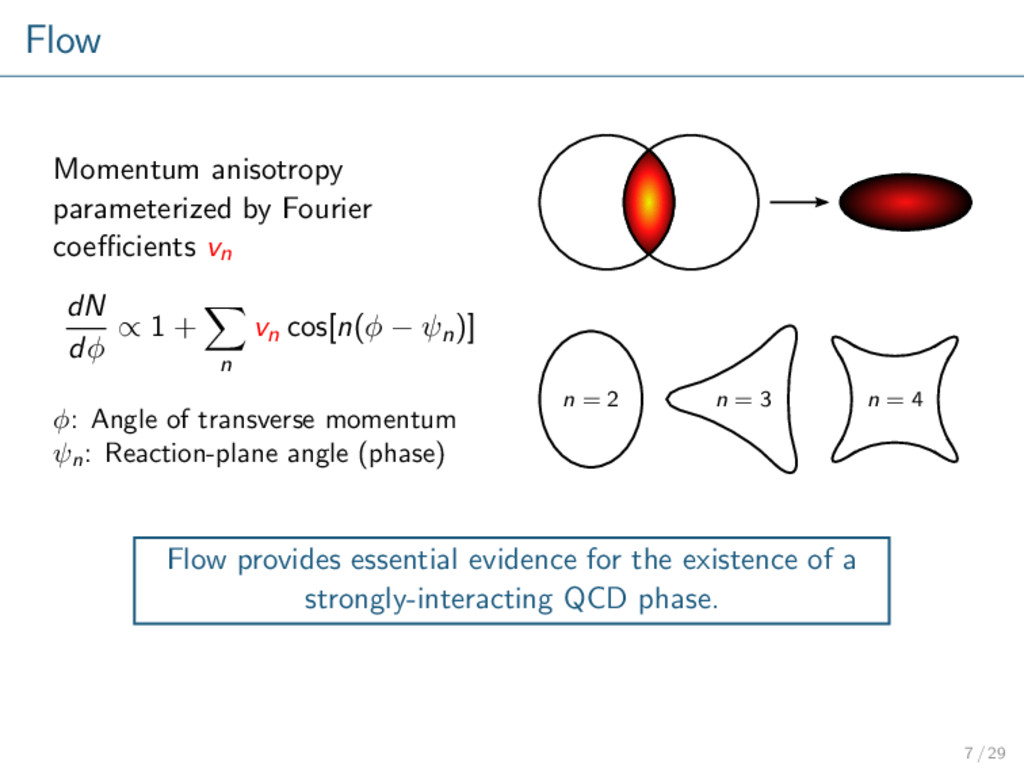
8. Flow Momentum anisotropy parameterized by Fourier coefficients vn dN dφ ∝ 1 + n vn cos[n(φ − ψn)] φ: Angle of transverse momentum ψn : Reaction-plane angle (phase) n = 2 n = 3 n = 4 Flow provides essential evidence for the existence of a strongly-interacting QCD phase. 7 / 29
9. Event-by-event fluctuations Average: symmetric nuclei, almond-shape overlap. Large v2 , small v4 , v6 , . . ., vanishing v3 , v5 , . . . Event-by-event: randomly distributed nucleons, irregular overlap. All vn nonzero. Flow probability distributions P(vn ). Average peripheral Fluctuating peripheral Fluctuating central 8 / 29
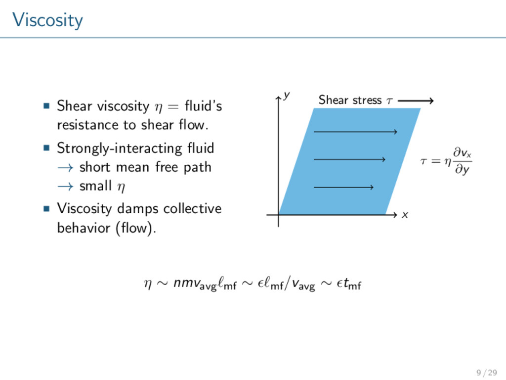
10. Viscosity Shear viscosity η = fluid’s resistance to shear flow. Strongly-interacting fluid → short mean free path → small η Viscosity damps collective behavior (flow). Shear stress τ x y τ = η ∂vx ∂y η ∼ nmvavg mf ∼ mf /vavg ∼ tmf 9 / 29
11. QGP specific shear viscosity Specific shear viscosity = dimensionless ratio to entropy density, η/s. η ∼ tmf , s ∼ n =⇒ η/s ∼ ( /n)tmf 1 Water η/s ∼ 300 at STP, Helium η/s ∼ 2 at 3 K, QGP η/s ∼ O(10−1). small η/s large v2 large η/s small v2 Measuring QGP η/s: Observe experimental vn. Run model with variable η/s. Constrain η/s by matching vn. 10 / 29
12. Simulations Modern event-by-event model: Monte Carlo initial conditions (Pre-equilibrium) Viscous relativistic hydrodynamics Monte Carlo freeze-out Boltzmann transport 11 / 29
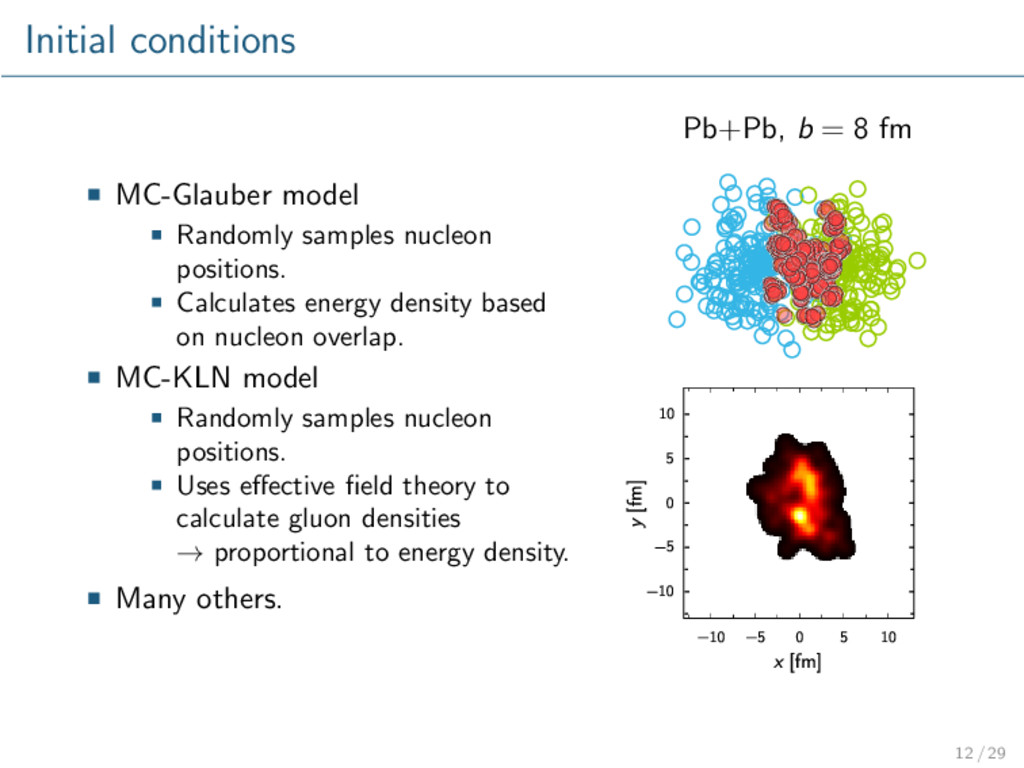
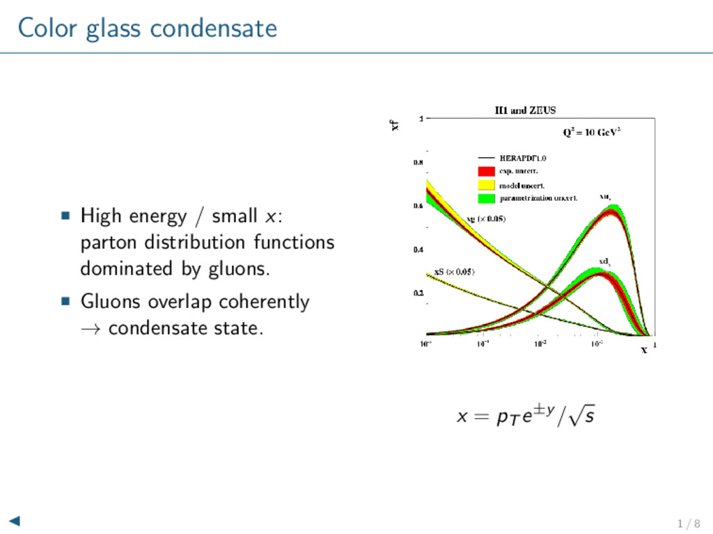
13. Initial conditions MC-Glauber model Randomly samples nucleon positions. Calculates energy density based on nucleon overlap. MC-KLN model Randomly samples nucleon positions. Uses effective field theory to calculate gluon densities → proportional to energy density. Many others. Pb+Pb, b = 8 fm 10 5 0 5 10 x [fm] 10 5 0 5 10 y [fm] 12 / 29
14. Viscous relativistic hydrodynamics Ignore pre-equilibrium, expand medium without interactions. Start hydro evolution at time τ0 (must set explicitly). Conservation equations: ∂µTµν = 0, Tµν = ( + P)uµuν − Pgµν + πµν. πµν contains dissipative effects (viscosity). Equation of state P = P( ). Initial condition Hydro η/s = 0.04 Hydro η/s = 0.24 10 5 0 5 10 x [fm] 10 5 0 5 10 y [fm] 10 5 0 5 10 x [fm] 10 5 0 5 10 x [fm] 40 80 120 160 Temperature [MeV] 13 / 29
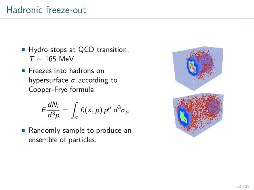
15. Hadronic freeze-out Hydro stops at QCD transition, T ∼ 165 MeV. Freezes into hadrons on hypersurface σ according to Cooper-Frye formula E dNi d3p = σ fi (x, p) pµ d3σµ Randomly sample to produce an ensemble of particles. 14 / 29
16. Transport Non-equilibrium Boltzmann transport dfi (x, p) dt = Ci (x, p) Calculates final collisions and decays. Particles stream into “detector”. 15 / 29
17. Model-to-data comparison: heavy-ion collisions Model Initial conditions, τ0, η/s, . . . 0.00 0.05 0.10 0.15 0.20 v2 0 5 10 15 20 P(v2 ) thick black line = ATLAS thin colored lines = model glb v2 20 25% 16 / 29
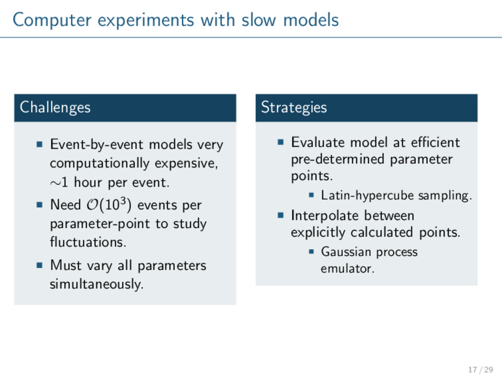
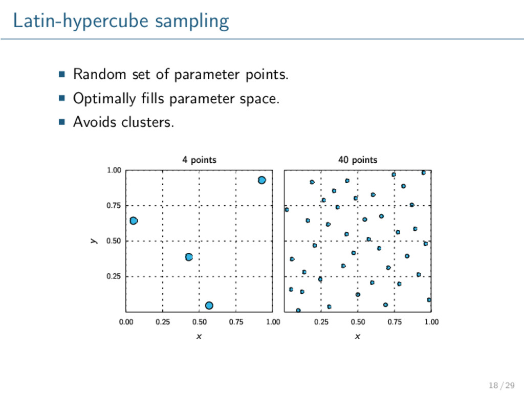
18. Computer experiments with slow models Challenges Event-by-event models very computationally expensive, ∼1 hour per event. Need O(103) events per parameter-point to study fluctuations. Must vary all parameters simultaneously. Strategies Evaluate model at efficient pre-determined parameter points. Latin-hypercube sampling. Interpolate between explicitly calculated points. Gaussian process emulator. 17 / 29
19. Latin-hypercube sampling Random set of parameter points. Optimally fills parameter space. Avoids clusters. 0.00 0.25 0.50 0.75 1.00 x 0.25 0.50 0.75 1.00 y 4 points 0.25 0.50 0.75 1.00 x 40 points 18 / 29
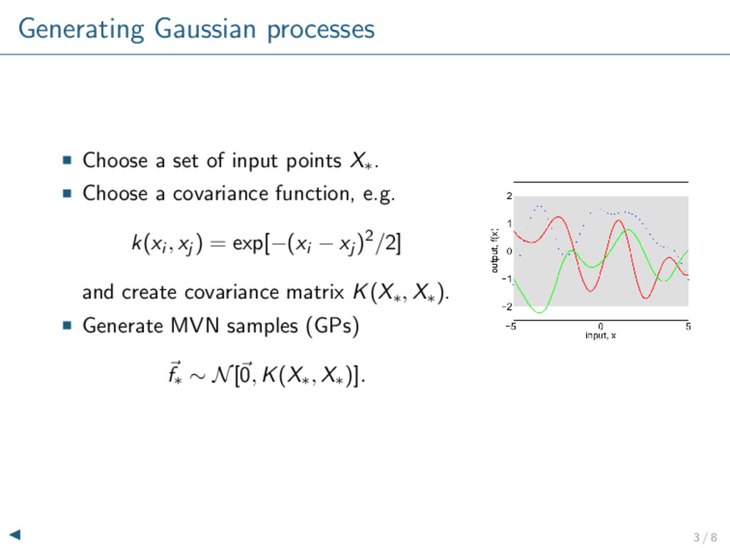
20. Gaussian processes A Gaussian process is a collection of random variables, any finite number of which have a joint Gaussian distribution. Instead of drawing variables from a distribution, functions are drawn from a process. Require a covariance function, e.g. cov(x1 , x2) ∝ exp − (x1 − x2)2 2 2 Nearby points correlated, distant points independent. Gaussian Processes for Machine Learning, Rasmussen and Williams, 2006. 19 / 29
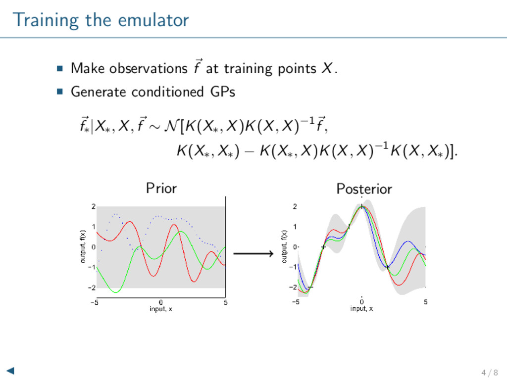
21. Gaussian process emulators Prior: the model is a Gaussian process. Posterior: Gaussian process conditioned on model outputs. Training Prior Posterior Emulator is a fast surrogate to the actual model. More certain near calculated points. Less certain in gaps. 20 / 29
22. Experimental data ATLAS event-by-event flow distributions v2 , v3 , v4. Fit to Rice / Bessel-Gaussian distribution P(vn) = vn δ2 vn e −(vn)2+(vRP n )2 2δ2 vn I0 vRP n vn δ2 vn Reduce to parameters vRP n , δvn . ATLAS Collaboration, JHEP 1311, 183 (2013). 21 / 29
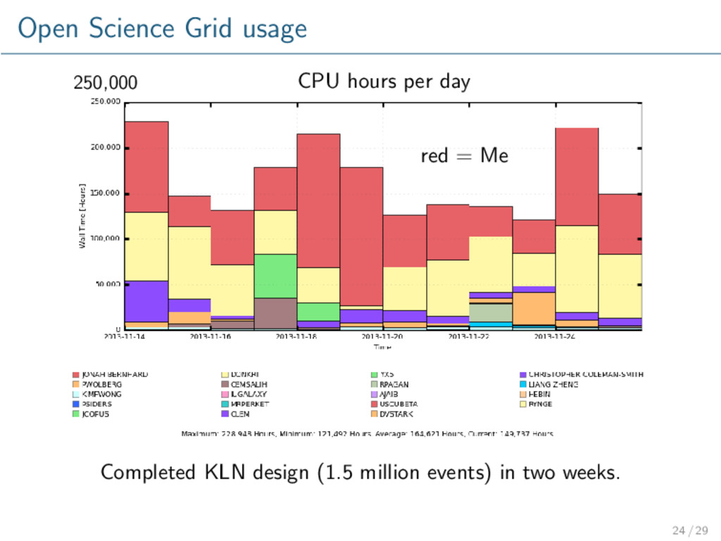
23. Event-by-event model Modern version of Duke+OSU model VISHNU (Viscous Hydro and UrQMD): MC-Glauber & MC-KLN initial conditions H.-J. Drescher and Y. Nara, Phys. Rev. C 74, 044905 (2006). Viscous hydro H. Song and U. Heinz, Phys. Rev. C 77, 064901 (2008). Cooper-Frye sampler Z. Qiu and C. Shen, arXiv:1308.2182 [nucl-th]. UrQMD (Ultrarelativistic Quantum Molecular Dynamics) S. Bass et. al., Prog. Part. Nucl. Phys. 41, 255 (1998). M. Bleicher et. al., J. Phys. G 25, 1859 (1999). → Tailored for running many events on Open Science Grid. 22 / 29
24. Computer experiment design Six centrality bins 0–5%, 10–15%, . . . 50–55%. 256 Latin-hypercube points, five input parameters: Normalization IC-specific parameter Thermalization time τ0 Viscosity η/s Shear relaxation time τΠ Massive parallelization on Open Science Grid. Completed 1000–2000 events per centrality bin and input-parameter point. 3.5 million total 0.5 µb−1 (ATLAS: 7 µb−1) 23 / 29
25. Open Science Grid usage CPU hours per day 250,000 red = Me Completed KLN design (1.5 million events) in two weeks. 24 / 29
26. Model flow distributions 0 5 10 15 20 25 30 35 P(v2 ) Glauber v2 00 05% thick black line = ATLAS thin colored lines = model KLN v2 00 05% 0.00 0.05 0.10 0.15 0.20 0.25 v2 0 2 4 6 8 10 12 14 16 P(v2 ) Glauber v2 40 45% 0.00 0.05 0.10 0.15 0.20 0.25 v2 KLN v2 40 45% 25 / 29
27. Input-output summary 0.04 0.08 vRP 2 0.015 0.030 v2 0.04 0.08 v2 0.015 0.030 v2 25 50 Normalization 0.3 0.4 v2 / v2 0.1 0.2 0.3 0.4 0.8 0 0.0 0.2 /s 0.4 0.8 Glauber v2 20 25% model trend ATLAS 26 / 29
28. Input-output summary 0.09 0.12 vRP 2 0.024 0.032 v2 0.09 0.12 v2 0.024 0.032 v2 8 12 Normalization 0.25 0.30 v2 / v2 0.16 0.24 0.4 0.8 0 0.0 0.2 /s 0.4 0.8 KLN v2 20 25% model trend ATLAS 26 / 29
29. Best parameter points Best Latin-hypercube points by average vn 0.00 0.02 0.04 0.06 0.08 0.10 0.12 0.14 vn Glauber /s=0.03 ATLAS v2 v3 v4 00-05 05-10 10-15 15-20 20-25 25-30 30-35 35-40 40-45 45-50 50-55 55-60 60-65 65-70 Centrality 0.00 0.02 0.04 0.06 0.08 0.10 0.12 0.14 vn KLN /s=0.21 OSU results, same model dashed: Glauber η/s = 0.08 solid: KLN η/s = 0.20 0 10 20 30 40 50 60 70 0 0.02 0.04 0.06 0.08 0.1 0.12 Centrality (%) vn ALICE v2 {2} ALICE v2 {4} ALICE v3 {2} ALICE v3 {4} MC-KLN MC-Glb. v2 v3 Z. Qiu, C. Shen, and U. Heinz, Phys. Lett. B 707, 151 (2012). 27 / 29
30. Constraining η/s Points: average η/s of best 10 Latin-hypercube points by average vn Error bars: standard deviation of best 10 Dashed lines: canonical η/s (Glauber 0.08, KLN 0.20) 00-05 05-10 10-15 15-20 20-25 25-30 30-35 35-40 40-45 45-50 50-55 Centrality 0.00 0.05 0.10 0.15 0.20 0.25 0.30 Preferred /s Glauber v2 v3 v4 00-05 05-10 10-15 15-20 20-25 25-30 30-35 35-40 40-45 45-50 50-55 Centrality KLN 28 / 29
31. Summary & outlook Framework for massive event-by-event model-to-data comparison: new level of knowledge-extraction capability. Preliminary results consistent with previous work. Improve goodness of fit: beyond average flow. Emulator: vary single parameters independently, determine best-fit parameter values. Calibrate simultaneously on other observables, e.g. multiplicity. Repeat with more advanced models, especially initial conditions. 29 / 29
32. backup slides
33. Color glass condensate High energy / small x: parton distribution functions dominated by gluons. Gluons overlap coherently → condensate state. x = pT e±y / √ s 1 / 8
34. Viscous hydro Conservation of energy and momentum: ∂µTµν = 0 Stress-energy tensor: Tµν = Tµν ideal + πµν Ideal part: Tµν ideal = ( + P)uµuν − Pgµν Shear viscosity correction: πµν = η∇ µuν Symmetric and traceless: ∇ µuν = ∇µuν + ∇νuµ − 2 3 ∆µν∇αuα Projection orthogonal to four velocity: ∆µν = gµν − uµuν ∇µ = ∆α µ ∂α 2 / 8
35. Generating Gaussian processes Choose a set of input points X∗. Choose a covariance function, e.g. k(xi , xj ) = exp[−(xi − xj )2/2] and create covariance matrix K(X∗ , X∗). Generate MVN samples (GPs) f∗ ∼ N[0, K(X∗ , X∗)]. 3 / 8
36. Training the emulator Make observations f at training points X. Generate conditioned GPs f∗ |X∗ , X, f ∼ N[K(X∗ , X)K(X, X)−1f , K(X∗ , X∗) − K(X∗ , X)K(X, X)−1K(X, X∗)]. Prior Posterior 4 / 8
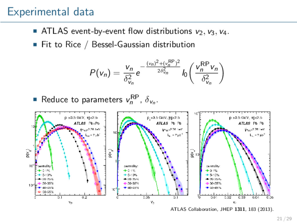
37. Rice / Bessel-Gaussian distribution Flow vectors follow bivariate Gaussian P(vn) = 1 2πδ2 vn e −(vn−vRP n )2 2δ2 vn . Integrate out angle P(vn) = vn δ2 vn e −(vn)2+(vRP n )2 2δ2 vn I0 vRP n vn δ2 vn . obs 2,x v -0.2 0 0.2 obs 2,y v -0.2 0 0.2 0 500 1000 centrality: 20-25% ATLAS Pb+Pb =2.76 TeV NN s -1 b µ = 7 int L |<2.5 η >0.5 GeV,| T p obs 2 v 0 0.1 0.2 0.3 Events 1 10 2 10 3 10 4 10 |<2.5 η >0.5 GeV,| T p ATLAS Pb+Pb =2.76 TeV NN s -1 b µ = 7 int L centrality: 20-25% 5 / 8
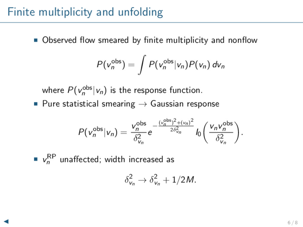
38. Finite multiplicity and unfolding Observed flow smeared by finite multiplicity and nonflow P(vobs n ) = P(vobs n |vn)P(vn) dvn where P(vobs n |vn) is the response function. Pure statistical smearing → Gaussian response P(vobs n |vn) = vobs n δ2 vn e −(vobs n )2+(vn)2 2δ2 vn I0 vnvobs n δ2 vn . vRP n unaffected; width increased as δ2 vn → δ2 vn + 1/2M. 6 / 8
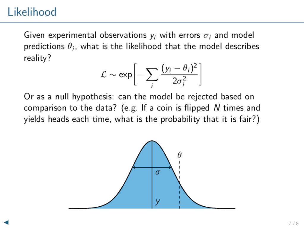
39. Likelihood Given experimental observations yi with errors σi and model predictions θi , what is the likelihood that the model describes reality? L ∼ exp − i (yi − θi )2 2σ2 i Or as a null hypothesis: can the model be rejected based on comparison to the data? (e.g. If a coin is flipped N times and yields heads each time, what is the probability that it is fair?) y σ θ 7 / 8
40. Linear fit example 0.00 0.02 0.04 0.06 0.08 0.10 0.12 0.001Norm + 0.130 + 0.026 0 0.062 /s + 0.020 0.00 0.02 0.04 0.06 0.08 0.10 0.12 v2 R2 ∼ 0.97 Glauber v2 20 25% 8 / 8