GBR 2011

Partial Diﬀerence Equations (PdE) on graphs for image and data
processing Olivier L´ ezoray Universit´ e de Caen Basse Normandie [email protected] http://www.info.unicaen.fr/~lezoray/ May 18, 2011 Joint work with A. Elmoataz.

1 Introduction 2 Graphs and diﬀerence operators 3 Construction of
graphs - non locality 4 p-Laplacian nonlocal regularization on graphs 5 Adaptive mathematical morphology on graphs 6 Eikonal equation on graphs 7 Conclusions & Actual Works O. L´ ezoray (University of Caen) PdE on graphs for image and data processing May 18, 2011 2 / 58

A deluge of many different kinds of data Different organization
Images Videos Meshes Social, complex, biological Networks ... And databases of them Different nature High dimensions, Non-linear, Heterogeneous, Noisy, redundant, incomplete O. L´ ezoray (University of Caen) PdE on graphs for image and data processing May 18, 2011 4 / 58

From image and data to graphs Graphs occur as a
the most natural of representing arbitrary data by modeling the neighborhood properties between these data (organized or not). 0.0 0.2 0.4 0.6 0.8 1.0 0.0 0.2 0.4 0.6 0.8 1.0 O. L´ ezoray (University of Caen) PdE on graphs for image and data processing May 18, 2011 5 / 58

the most natural of representing arbitrary data by modeling the neighborhood properties between these data (organized or not). 0.0 0.2 0.4 0.6 0.8 1.0 0.0 0.2 0.4 0.6 0.8 1.0 Images, Region adjacency graphs O. L´ ezoray (University of Caen) PdE on graphs for image and data processing May 18, 2011 5 / 58

the most natural of representing arbitrary data by modeling the neighborhood properties between these data (organized or not). 0.0 0.2 0.4 0.6 0.8 1.0 0.0 0.2 0.4 0.6 0.8 1.0 0.0 0.2 0.4 0.6 0.8 1.0 0.0 0.2 0.4 0.6 0.8 1.0 Points clouds, meshes O. L´ ezoray (University of Caen) PdE on graphs for image and data processing May 18, 2011 5 / 58

the most natural of representing arbitrary data by modeling the neighborhood properties between these data (organized or not). 0.0 0.2 0.4 0.6 0.8 1.0 0.0 0.2 0.4 0.6 0.8 1.0 Image databases O. L´ ezoray (University of Caen) PdE on graphs for image and data processing May 18, 2011 5 / 58

Typical problems in image and data processing Given some input
Data X0 , we want to conceive a processing operator Υ that outputs the processed data X1 . Typical processing operators Restoration, denoising, interpolation Smoothing, simpliﬁcation Segmentation, classiﬁcation Dimensionality reduction Visualization, exploration O. L´ ezoray (University of Caen) PdE on graphs for image and data processing May 18, 2011 6 / 58

Data X0 , we want to conceive a processing operator Υ that outputs the processed data X1 . Typical processing operators Restoration, denoising, interpolation Smoothing, simpliﬁcation Segmentation, classiﬁcation Dimensionality reduction Visualization, exploration Two problems arise How to model and represent the input and output data sources ? How to model and formalize the processing operator ? O. L´ ezoray (University of Caen) PdE on graphs for image and data processing May 18, 2011 6 / 58

Data X0 , we want to conceive a processing operator Υ that outputs the processed data X1 . Typical processing operators Restoration, denoising, interpolation Smoothing, simplification Segmentation, classification Dimensionality reduction Visualization, exploration Two problems arise How to model and represent the input and output data sources ? How to model and formalize the processing operator ? Different methods to do this Graph theory, spectral analysis (Mainly for data processing) Continuous variational methods (Mainly for image processing) A lot of new works aim at extending signal processing for data processing (e.g, diffusion wavelets) Partial difference Equations on graphs (a unified framework for image and data processing) O. L´ ezoray (University of Caen) PdE on graphs for image and data processing May 18, 2011 6 / 58

Continuous variational methods Benefits Provide a formal framework for the
resolution of problems in image processing, computer vision, etc. Solutions are obtained by the minimization of appropriate energy functions The minimization is usually performed with Partial Differential Equations (PDEs) PDEs are discretized to obtain a numerical solution Limitations PDE-based methods are difficult to adapt for data that live on non Euclidean domains Indeed, their discretization is difficult for high dimensional data Not easy to extend them to advanced representations of data, i.e., graphs It is essential to be able to transcript PDEs on graphs O. L´ ezoray (University of Caen) PdE on graphs for image and data processing May 18, 2011 7 / 58

Partial difference Equations on graphs Motivations Problems involving PDEs can
be reduced to ones of a very much simpler structure by replacing the differentials by difference equations on graphs. R. Courant, K. Friedrichs, H. Lewy, On the partial difference equations of mathematical physics, Math. Ann. 100 (1928) 32-74. Our goal is to provide methods that mimic on graphs well-known PDE variational formulations under a functional analysis point of view. To do this we use Partial difference Equations (PdE) over graphs. PdEs mimic PDEs in domains having a graph structure. Interest of our proposals To dispose of discrete analogues of differential geometry operators (integral, derivation, gradient, divergence, p-Laplacian, etc.) To use the framework of PdEs to transcribe PDEs on graphs, Provides a natural extension of variational methods on graphs, Provides a unification of local and nonlocal processing on images. Using weighted graphs provides Adaptive PDEs according to data geometry O. L´ ezoray (University of Caen) PdE on graphs for image and data processing May 18, 2011 8 / 58

What we will talk about a nonlocal discrete regularization on
graphs as a framework for data simpliﬁcation and interpolation, a formulation of mathematical morphology that considers a discrete version of PDEs-based approaches over weighted graphs, an adaptation of the Eikonal equation for data clustering and image segmentation. O. L´ ezoray (University of Caen) PdE on graphs for image and data processing May 18, 2011 9 / 58

Weighted graphs Basics A weighted graph G = (V, E,
w) consists in a ﬁnite set V = {v1, . . . , vN } of N vertices O. L´ ezoray (University of Caen) PdE on graphs for image and data processing May 18, 2011 11 / 58

w) consists in a ﬁnite set V = {v1, . . . , vN } of N vertices and a ﬁnite set E = {e1, . . . , eN } ⊂ V × V of N weighted edges. We assume G to be simple, undirected, with no self-loops and no multiple edges. O. L´ ezoray (University of Caen) PdE on graphs for image and data processing May 18, 2011 11 / 58

w) consists in a ﬁnite set V = {v1, . . . , vN } of N vertices and a ﬁnite set E = {e1, . . . , eN } ⊂ V × V of N weighted edges. We assume G to be simple, undirected, with no self-loops and no multiple edges. eij = (vi , vj ) is the edge of E that connects vertices vi and vj of V. Its weight, denoted by wij = w(vi , vj ), represents the similarity between its vertices. Similarities are usually computed by using a positive symmetric function w : V × V → R+ satisfying w(vi , vj ) = 0 if (vi , vj ) / ∈ E. w w w w w w w w w w w O. L´ ezoray (University of Caen) PdE on graphs for image and data processing May 18, 2011 11 / 58

w) consists in a ﬁnite set V = {v1, . . . , vN } of N vertices and a ﬁnite set E = {e1, . . . , eN } ⊂ V × V of N weighted edges. We assume G to be simple, undirected, with no self-loops and no multiple edges. eij = (vi , vj ) is the edge of E that connects vertices vi and vj of V. Its weight, denoted by wij = w(vi , vj ), represents the similarity between its vertices. Similarities are usually computed by using a positive symmetric function w : V × V → R+ satisfying w(vi , vj ) = 0 if (vi , vj ) / ∈ E. The notation vi ∼ vj is used to denote two adjacent vertices. O. L´ ezoray (University of Caen) PdE on graphs for image and data processing May 18, 2011 11 / 58

Space of functions on Graphs Let H(V) be the Hilbert
space of real-valued functions defined on the vertices of a graph. A function f : V → R of H(V) assigns a real value xi = f (vi ) to each vertex vi ∈ V. By analogy with functional analysis on continuous spaces, the integral of a function f ∈ H(V), over the set of vertices V, is defined as V f = V f . The space H(V) is endowed with the usual inner product f , h H(V) = vi ∈V f (vi )h(vi ), where f , h : V → R. Similarly, let H(E) be the space of real-valued functions defined on the edges of G. It is endowed with the inner product F, H H(E) vi ∈V vj ∼vi F(vi , vj )H(vi , vj ), where F, H : E → R are two functions of H(E). O. L´ ezoray (University of Caen) PdE on graphs for image and data processing May 18, 2011 12 / 58

Difference operators on weighted graphs · Discretization of classical continuous
differential geometry. The difference operator of f , dw : H(V) → H(E), is defined on an edge eij = (vi , vj ) ∈ E by: (dw f )(eij ) = (dw f )(vi , vj ) = w(vi , vj )1/2(f (vj ) − f (vi )) . (1) The adjoint of the difference operator, noted d∗ w : H(E) → H(V), is a linear operator defined by dw f , H H(E) = f , d∗ w H H(V) for all f ∈ H(V) and all H ∈ H(E). The adjoint operator d∗ w , of a function H ∈ H(E), can by expressed at a vertex vi ∈ V by the following expression: (d∗ w H)(vi ) = −divw (H)(vi ) = vj ∼vi w(vi , vj )1/2(H(vj , vi ) − H(vi , vj )) . (2) Each function H ∈ H(E) has a null divergence over the entire set of vertices: vi ∈V (d∗ w H)(vi ) = 0. O. L´ ezoray (University of Caen) PdE on graphs for image and data processing May 18, 2011 13 / 58

Difference operators on weighted graphs The directional derivative (or edge
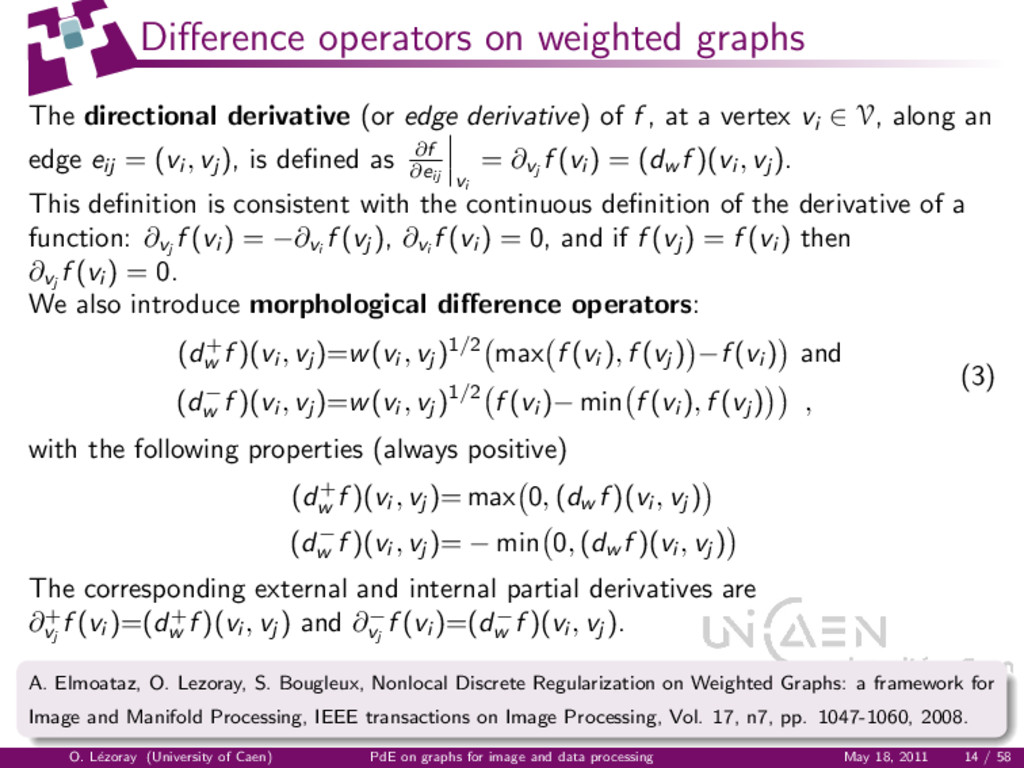
derivative) of f , at a vertex vi ∈ V, along an edge eij = (vi , vj ), is defined as ∂f ∂eij vi = ∂vj f (vi ) = (dw f )(vi , vj ). This definition is consistent with the continuous definition of the derivative of a function: ∂vj f (vi ) = −∂vi f (vj ), ∂vi f (vi ) = 0, and if f (vj ) = f (vi ) then ∂vj f (vi ) = 0. We also introduce morphological difference operators: (d+ w f )(vi , vj )=w(vi , vj )1/2 max f (vi ), f (vj ) −f (vi ) and (d− w f )(vi , vj )=w(vi , vj )1/2 f (vi )− min f (vi ), f (vj ) , (3) with the following properties (always positive) (d+ w f )(vi , vj )= max 0, (dw f )(vi , vj ) (d− w f )(vi , vj )= − min 0, (dw f )(vi , vj ) The corresponding external and internal partial derivatives are ∂+ vj f (vi )=(d+ w f )(vi , vj ) and ∂− vj f (vi )=(d− w f )(vi , vj ). A. Elmoataz, O. Lezoray, S. Bougleux, Nonlocal Discrete Regularization on Weighted Graphs: a framework for Image and Manifold Processing, IEEE transactions on Image Processing, Vol. 17, n7, pp. 1047-1060, 2008. O. L´ ezoray (University of Caen) PdE on graphs for image and data processing May 18, 2011 14 / 58

Weighted gradient operator The weighted gradient operator of a function
f ∈ H(V), at a vertex vi ∈ V, is the vector operator deﬁned by (∇w f)(vi ) = [∂vj f (vi ) : vj ∼ vi ]T = [∂v1 f (vi ), . . . , ∂vk f (vi )]T , ∀(vi , vj ) ∈ E. (4) The Lp norm of this vector represents the local variation of the function f at a vertex of the graph (It is a semi-norm for p ≥ 1): (∇w f)(vi ) p = vj ∼vi wp/2 ij f (vj )−f (vi ) p 1/p . (5) Similarly, we have with M+ = max and M− = min (∇± w f)(vi )= ∂± vj f (vi ) T (vi ,vj )∈E . (∇± w f)(vi ) p = vj ∼vi w(vi , vj )p/2 M± 0, f (vj )−f (vi ) p 1/p . (6) O. L´ ezoray (University of Caen) PdE on graphs for image and data processing May 18, 2011 15 / 58

Isotropic p-Laplacian The weighted p-Laplace isotropic operator of a function
f ∈ H(V), noted ∆i w,p : H(V) → H(V), is deﬁned by: (∆i w,p f )(vi ) = 1 2 d∗ w ( (∇w f)(vi ) p−2 2 (dw f )(vi , vj )) . (7) The isotropic p-Laplace operator of f ∈ H(V), at a vertex vi ∈ V, can be computed by: (∆i w,p f )(vi ) = 1 2 vj ∼vi (γi w,p f )(vi , vj )(f (vi ) − f (vj )) , (8) with (γi w,p f )(vi , vj ) = wij (∇w f)(vj ) p−2 2 + (∇w f)(vi ) p−2 2 . (9) The p-Laplace isotropic operator is nonlinear, except for p = 2 (corresponds to the combinatorial Laplacian). For p = 1, it corresponds to the weighted curvature of the function f on the graph. A. Elmoataz, O. Lezoray, S. Bougleux, Nonlocal Discrete Regularization on Weighted Graphs: a framework for Image and Manifold Processing, IEEE transactions on Image Processing, Vol. 17, n7, pp. 1047-1060, 2008. O. L´ ezoray (University of Caen) PdE on graphs for image and data processing May 18, 2011 16 / 58

Anisotropic p-Laplacian The weighted p-Laplace anisotropic operator of a function
f ∈ H(V), noted ∆a w,p : H(V) → H(V), is defined by: (∆a w,p f )(vi ) = 1 2 d∗ w (|(dw f )(vi , vj )|p−2(dw f )(vi , vj )) . (10) The anisotropic p-Laplace operator of f ∈ H(V), at a vertex vi ∈ V, can be computed by: (∆a w,p f )(vi ) = vj ∼vi (γa w,p f )(vi , vj )(f (vi ) − f (vj )) . (11) with (γa w,p f )(vi , vj ) = wp/2 ij |f (vi ) − f (vj )|p−2 . (12) O. Lezoray, V.T. Ta, A. Elmoataz, Partial differences as tools for filtering data on graphs, Pattern Recognition Letters, Vol. 31, n14, pp. 2201-2213, 2010. O. L´ ezoray (University of Caen) PdE on graphs for image and data processing May 18, 2011 17 / 58

Constructing graphs Any discrete domain can be modeled by a
weighted graph where each data point is represented by a vertex vi ∈ V. Unorganized data An unorganized set of points V ⊂ Rn can be seen as a function f 0 : V → Rm. The set of edges is deﬁned by in modeling the neighborhood of each vertex based on similarity relationships between feature vectors. Typical graphs: k-nearest neighbors graphs and τ-neighborhood graphs. Organized data Typical cases of organized data are signals, gray-scale or color images (in 2D or 3D). The set of edge is deﬁned by spatial relationships. Such data can be seen as functions f 0 : V ⊂ Zn → Rm. Typical graphs: pixel or region graphs. 12 2 — GRAPHES ET OPÉRATEURS ! !! ! ! ! ! !! ! ! ! ! ! ! ! ! ! ! ! ! ! ! ! ! ! ! ! ! ! ! ! ! ! ! ! ! ! ! ! ! ! ! ! ! ! ! ! ! ! ! ! ! ! !! ! ! ! ! !! ! ! ! ! ! ! !! ! !! ! !!! !! ! ! ! ! !! ! ! ! !! ! ! !! ! ! ! ! ! ! ! ! ! ! ! ! ! ! ! ! ! ! ! ! ! ! ! ! ! ! ! ! ! ! ! ! ! ! ! ! ! ! ! ! ! ! ! ! ! ! ! ! ! ! ! ! ! ! ! ! ! ! ! ! ! ! ! ! ! ! ! ! ! ! ! ! ! ! ! ! ! ! ! ! ! ! ! ! ! ! ! ! ! ! ! ! ! ! ! ! ! ! ! ! ! ! ! ! ! ! 0.0 0.2 0.4 0.6 0.8 1.0 0.0 0.2 0.4 0.6 0.8 1.0 (a) ! !! ! ! ! ! !! ! ! ! ! ! ! ! ! ! ! ! ! ! ! ! ! ! ! ! ! ! ! ! ! ! ! ! ! ! ! ! ! ! ! ! ! ! ! ! ! ! ! ! ! ! !! ! ! ! ! !! ! ! ! ! ! ! !! ! !! ! !!! !! ! ! ! ! !! ! ! ! !! ! ! !! ! ! ! ! ! ! ! ! ! ! ! ! ! ! ! ! ! ! ! ! ! ! ! ! ! ! ! ! ! ! ! ! ! ! ! ! ! ! ! ! ! ! ! ! ! ! ! ! ! ! ! ! ! ! ! ! ! ! ! ! ! ! ! ! ! ! ! ! ! ! ! ! ! ! ! ! ! ! ! ! ! ! ! ! ! ! ! ! ! ! ! ! ! ! ! ! ! ! ! ! ! ! ! ! ! ! 0.0 0.2 0.4 0.6 0.8 1.0 0.0 0.2 0.4 0.6 0.8 1.0 (b) k=3 ! !! ! ! ! ! !! ! ! ! ! ! ! ! ! ! ! ! ! ! ! ! ! ! ! ! ! ! ! ! ! ! ! ! ! ! ! ! ! ! ! ! ! ! ! ! ! ! ! ! ! ! !! ! ! ! ! !! ! ! ! ! ! ! !! ! !! ! !!! !! ! ! ! ! !! ! ! ! !! ! ! !! ! ! ! ! ! ! ! ! ! ! ! ! ! ! ! ! ! ! ! ! ! ! ! ! ! ! ! ! ! ! ! ! ! ! ! ! ! ! ! ! ! ! ! ! ! ! ! ! ! ! ! ! ! ! ! ! ! ! ! ! ! ! ! ! ! ! ! ! ! ! ! ! ! ! ! ! ! ! ! ! ! ! ! ! ! ! ! ! ! ! ! ! ! ! ! ! ! ! ! ! ! ! ! ! ! ! 0.0 0.2 0.4 0.6 0.8 1.0 0.0 0.2 0.4 0.6 0.8 1.0 (c) k=15 Fig. 2.1 – Exemples de graphes des k plus proches voisins. (a) : données initiales dans IR2, (b) : 3-Nng, (c) : 15-Nng. O. L´ ezoray (University of Caen) PdE on graphs for image and data processing May 18, 2011 19 / 58

Weighting graphs For an initial function f 0 : V
→ Rm, similarity relationship between data can be incorporated within edges weights according to a measure of similarity g : E → [0, 1] with w(eij ) = g(eij ), ∀eij ∈ E. Each vertex vi is associated with a feature vector Ff0 τ : V → Rm×q where q corresponds to this vector size: Ff0 τ (vi ) = f 0(vj ) : vj ∈ Nτ (vi ) ∪ {vi } T (13) with Nτ (vi ) = vj ∈ V \ {vi } : µ(vi , vj ) ≤ τ . For an edge eij and a distance measure ρ : Rm×q×Rm×q → R associated to Ff0 τ , we can have: g1 (eij ) =1 (unweighted case) , g2 (eij ) = exp −ρ Ff0 τ (vi ), Ff0 τ (vj ) 2/σ2 with σ > 0 , g3 (eij ) =1/ 1 + ρ Ff0 τ (vi ), Ff0 τ (vj ) (14) O. L´ ezoray (University of Caen) PdE on graphs for image and data processing May 18, 2011 20 / 58

Local to Non Local to Graphs In Image Processing, we
can divide methods according to three diﬀerent models: Local Processing: usual model where local interactions around one pixel are taken into account (Vector Median Filter, Anisotropic Filtering, Wavelets, Total Variation minimization with PDE, etc.), O. L´ ezoray (University of Caen) PdE on graphs for image and data processing May 18, 2011 21 / 58

can divide methods according to three diﬀerent models: Local Processing: usual model where local interactions around one pixel are taken into account (Vector Median Filter, Anisotropic Filtering, Wavelets, Total Variation minimization with PDE, etc.), Semi Local Processing: one takes into account larger neighborhood interactions favored by the image geometry (Yaroslavsky and Bilateral ﬁlters), O. L´ ezoray (University of Caen) PdE on graphs for image and data processing May 18, 2011 21 / 58

can divide methods according to three diﬀerent models: Local Processing: usual model where local interactions around one pixel are taken into account (Vector Median Filter, Anisotropic Filtering, Wavelets, Total Variation minimization with PDE, etc.), Semi Local Processing: one takes into account larger neighborhood interactions favored by the image geometry (Yaroslavsky and Bilateral ﬁlters), Non Local Processing: model recently proposed by Buades and Morel which replaces spatial constraints by pixel blocks (i.e. patchs) constraints in a large neighborhood. O. L´ ezoray (University of Caen) PdE on graphs for image and data processing May 18, 2011 21 / 58

can divide methods according to three diﬀerent models: Local Processing: usual model where local interactions around one pixel are taken into account (Vector Median Filter, Anisotropic Filtering, Wavelets, Total Variation minimization with PDE, etc.), Semi Local Processing: one takes into account larger neighborhood interactions favored by the image geometry (Yaroslavsky and Bilateral ﬁlters), Non Local Processing: model recently proposed by Buades and Morel which replaces spatial constraints by pixel blocks (i.e. patchs) constraints in a large neighborhood. w O. L´ ezoray (University of Caen) PdE on graphs for image and data processing May 18, 2011 21 / 58

Graph topology Digital Image

Graph topology Digital Image 8-neighborhood : 3 × 3

Graph topology Digital Image 8-neighborhood : 3 × 3 24-neighborhood
: 5 × 5

: 5 × 5 Local: a value is associated to vertices

: 5 × 5 Local: a value is associated to vertices Nonlocal: a patch (vector of values in a given neighborhood) is associated to vertices. O. L´ ezoray (University of Caen) PdE on graphs for image and data processing May 18, 2011 22 / 58

: 5 × 5 Local: a value is associated to vertices Nonlocal: a patch (vector of values in a given neighborhood) is associated to vertices. With Graphs Nonlocal behavior is directly expressed by the graph topology. Patches are used to measure similarity between vertices. O. L´ ezoray (University of Caen) PdE on graphs for image and data processing May 18, 2011 22 / 58

: 5 × 5 Local: a value is associated to vertices Nonlocal: a patch (vector of values in a given neighborhood) is associated to vertices. Consequences Nonlocal processing of images becomes local processing on similarity graphs. Our diﬀerence operators on graphs naturally enable local and nonlocal conﬁgurations (with the weight function and the graph topology) O. L´ ezoray (University of Caen) PdE on graphs for image and data processing May 18, 2011 22 / 58

p-Laplacian nonlocal regularization on graphs Let f 0 : V
→ R be a given (noisy) function deﬁned on the vertices of a weighted graph G = (V, E, w). f 0 represents an observation of a clean function g : V → R corrupted by a given noise n such that f 0 = g + n. Recovering the uncorrupted function g is an inverse problem: a commonly used method is to seek for a function f : V → R which is regular enough on G, and also close enough to f 0. We consider the following variational problem: g ≈ min f :V→R E∗ w,p (f , f 0, λ) = R∗ w,p (f ) + λ 2 f − f 0 2 2 , (15) where the regularization functional R∗ w,p : H(V) → R can correspond to an isotropic Ri w,p or an anisotropic Ra w,p functionnal. A. Elmoataz, O. Lezoray, S. Bougleux, Nonlocal Discrete Regularization on Weighted Graphs: a framework for Image and Manifold Processing, IEEE transactions on Image Processing, Vol. 17, n7, pp. 1047-1060, 2008. O. L´ ezoray (University of Caen) PdE on graphs for image and data processing May 18, 2011 24 / 58

Isotropic an anisotropic regularization terms The isotropic regularization functionnal Ri
w,p is deﬁned by the L2 norm of the gradient and is the discrete p-Dirichlet form of the function f ∈ H(V): Ri w,p (f ) = 1 p vi ∈V (∇w f)(vi ) p 2 = 1 p f , ∆i w,p f H(V) = 1 p vi ∈V   vj ∼vi wij (f (vj ) − f (vi ))2   p 2 . (16) The anisotropic regularization functionnal Ra w,p is deﬁned by the Lp norm of the gradient: Ra w,p (f ) = 1 p vi ∈V (∇w f)(vi ) p p = 1 p f , ∆a w,p f H(V) = 1 p vi ∈V vj ∼vi wp/2 ij |f (vj ) − f (vi )|p . (17) When p ≥ 1, the energy E∗ w,p is a convex functional of functions of H(V). O. L´ ezoray (University of Caen) PdE on graphs for image and data processing May 18, 2011 25 / 58

Isotropic diﬀusion process To get the solution of the minimizer,
we consider the following system of equations: ∂Ei w,p (f , f 0, λ) ∂f (vi ) = 0, ∀vi ∈ V (18) which is rewritten as: ∂Ri w,p (f ) ∂f (vi ) + λ(f (vi ) − f 0(vi )) = 0, ∀vi ∈ V. (19) Moreover, we can prove that ∂Ri w,p (f ) ∂f (vi ) = 2(∆i w,p f )(vi ) . (20) The system of equations is then rewritten as 2(∆i w,p f )(vi ) + λ(f (vi ) − f 0(vi )) = 0, ∀vi ∈ V, (21) which is equivalent to the following system of equations:  λ + vj ∼vi (γi w,p f )(vi , vj )   f (vi ) − vj ∼vi (γi w,p f )(vi , vj )f (vj ) = λf 0(vi ). (22) O. L´ ezoray (University of Caen) PdE on graphs for image and data processing May 18, 2011 26 / 58

Isotropic diﬀusion process We use the linearized Gauss-Jacobi iterative method
to solve the previous system. Let n be an iteration step, and let f (n) be the solution at the step n. Then, the method is given by the following algorithm:        f (0) = f 0 f (n+1)(vi ) = λf 0(vi ) + vj ∼vi (γi w,p f (n))(vi , vj )f (n)(vj ) λ + vj ∼vi (γi w,p f (n))(vi , vj ) , ∀vi ∈ V. (23) with (γi w,p f )(vi , vj ) = wij (∇w f)(vj ) p−2 2 + (∇w f)(vi ) p−2 2 . (24) It describes a family of discrete diﬀusion processes, which is parameterized by the structure of the graph (topology and weight function), the parameter p, and the parameter λ. λ w Graph p = 1 p = 2 p ∈]0, 1[ 0 exp() semi-local Our Bilateral Our 0 exp() nonlocal Our NLMeans Our = 0 constant local TV Digital L2 Digital Our = 0 any nonlocal Our Our Our Table: Works related to our framework in image processing. O. L´ ezoray (University of Caen) PdE on graphs for image and data processing May 18, 2011 27 / 58

Examples: Image denoising Original image Noisy image (Gaussian noise with
σ = 15) f 0 : V → R3 PSNR=29.38dB O. L´ ezoray (University of Caen) PdE on graphs for image and data processing May 18, 2011 28 / 58

Examples: Image denoising Isotropic G1 , Ff0 0 = f
0 Isotropic G7 , Ff0 3 Anisotropic G7 , Ff0 3 p = 2 PSNR=28.52db PSNR=31.79dB PSNR=31.79dB p = 1 PSNR=31.25dB PSNR=34.74dB PSNR=31.81dB O. L´ ezoray (University of Caen) PdE on graphs for image and data processing May 18, 2011 29 / 58

Examples: Image Database denoising Initial data Noisy data 10-NNG f
0 : V → R16×16 O. L´ ezoray (University of Caen) PdE on graphs for image and data processing May 18, 2011 30 / 58

Examples: Image Database denoising λ = 1 λ = 0.01
λ = 0 Isotropic p = 1 PSNR=18.80dB PSNR=13.54dB PSNR=10.52dB Anisotropic p = 1 PSNR=18.96dB PSNR=15.19dB PSNR=14.41dB O. L´ ezoray (University of Caen) PdE on graphs for image and data processing May 18, 2011 31 / 58

Interpolation of missing data on graphs Let f 0 :
V0 → R be a function with V0 ⊂ V be the subset of vertices from the whole graph with known values. The interpolation consists in recovering values of f for the vertices of V \ V0 given values for vertices of V0 formulated by: min f :V→R R∗ w,p (f ) + λ(vi ) f (vi ) − f 0(vi ) 2 2 . (25) Since f 0(vi ) is known only for vertices of V0 , the Lagrange parameter is deﬁned as λ : V → R: λ(vi ) = λ if vi ∈ V0 0 otherwise. (26) This comes to consider ∆∗ w,p f (vi ) = 0 on V \ V0 . Our isotropic and anisotropic diﬀusion processes can be directly used to perform the interpolation. O. L´ ezoray (University of Caen) PdE on graphs for image and data processing May 18, 2011 32 / 58

Examples: Image segmentation Original Image User label input Segmentation result
G0 , Ff0 0 = f 0, w = g2 , p = 2, λ = 1 G0 ∪ 4-NNG3 , Ff0 3 , w = g2 , p = 2, λ = 1 O. L´ ezoray (University of Caen) PdE on graphs for image and data processing May 18, 2011 33 / 58

Examples: Image segmentation (a) 27 512 pixels (b) Original+Labels (c)
t = 50 (11 seconds) (d) 639 zones (98% of reduction) (e) Original+Labels (f) t = 5 (< 1 second) (g) 639 zones (98% of reduction) (h) Original+Labels (i) t = 2 (< 1 second) O. L´ ezoray (University of Caen) PdE on graphs for image and data processing May 18, 2011 34 / 58

Examples: Data base clustering ! ! ! ! ! !
! ! ! ! ! ! !! ! ! ! ! ! ! ! ! ! ! ! ! ! ! ! !! ! ! ! ! ! ! ! ! ! ! ! ! ! ! ! ! ! ! ! ! ! ! ! ! !! ! ! ! ! ! ! ! ! ! ! ! !! ! ! ! ! ! ! ! ! ! ! ! ! ! ! ! ! ! ! ! ! ! ! ! ! ! ! ! ! !! ! ! ! ! ! ! ! ! ! ! ! ! ! ! ! ! ! ! ! ! ! ! ! ! ! ! ! ! ! ! ! ! ! ! ! ! ! ! ! 50 100 150 200 250 60 80 100 (a) Données initiales avec les marqueurs initiaux ! ! ! ! ! ! ! ! ! ! ! ! !! ! ! ! ! ! ! ! ! ! ! ! ! ! ! ! !! ! ! ! ! ! ! ! ! ! ! ! ! ! ! ! ! ! ! ! ! ! ! ! ! !! ! ! ! ! ! ! ! ! ! ! ! !! ! ! ! ! ! ! ! ! ! ! ! ! ! ! ! ! ! ! ! ! ! ! ! ! ! ! ! ! !! ! ! ! ! ! ! ! ! ! ! ! ! ! ! ! ! ! ! ! ! ! ! ! ! ! ! ! ! ! ! ! ! ! ! ! ! ! ! ! 50 100 150 200 250 60 80 100 (b) 20-Nng n = 1 n = 5 n = 10 ! ! ! ! ! ! ! ! ! ! ! ! !! ! ! ! ! ! ! ! ! ! ! ! ! ! ! ! !! ! ! ! ! ! ! ! ! ! ! ! ! ! ! ! ! ! ! ! ! ! ! ! ! !! ! ! ! ! ! ! ! ! ! ! ! !! ! ! ! ! ! ! ! ! ! ! ! ! ! ! ! ! ! ! ! ! ! ! ! ! ! ! ! ! !! ! ! ! ! ! ! ! ! ! ! ! ! ! ! ! ! ! ! ! ! ! ! ! ! ! ! ! ! ! ! ! ! ! ! ! ! ! ! ! ! ! ! ! ! ! ! ! ! ! ! ! ! ! ! ! ! ! ! ! ! ! ! ! !! ! ! ! ! ! ! ! ! ! ! ! ! ! ! ! !! ! ! ! ! ! ! ! ! ! ! ! ! ! ! ! ! ! ! ! ! ! ! ! ! ! ! ! ! ! ! ! ! ! !! ! ! ! ! ! ! ! ! ! ! ! ! !!! ! ! ! ! ! ! ! !! ! ! ! ! ! ! ! ! ! ! ! ! !! 50 100 150 200 250 60 80 100 120 140 160 180 200 ! ! ! ! ! ! ! ! ! ! ! ! !! ! ! ! ! ! ! ! ! ! ! ! ! ! ! ! !! ! ! ! ! ! ! ! ! ! ! ! ! ! ! ! ! ! ! ! ! ! ! ! ! !! ! ! ! ! ! ! ! ! ! ! ! !! ! ! ! ! ! ! ! ! ! ! ! ! ! ! ! ! ! ! ! ! ! ! ! ! ! ! ! ! !! ! ! ! ! ! ! ! ! ! ! ! ! ! ! ! ! ! ! ! ! ! ! ! ! ! ! ! ! ! ! ! ! ! ! ! ! ! ! ! ! ! ! ! ! ! ! ! ! ! ! ! ! ! ! ! ! ! ! ! ! ! ! ! !! ! ! ! ! ! ! ! ! ! ! ! ! ! ! ! !! ! ! ! ! ! ! ! ! ! ! ! ! ! ! ! ! ! ! ! ! ! ! ! ! ! ! 50 100 150 200 250 60 80 100 120 140 160 180 200 ! ! ! ! ! ! ! ! ! ! ! ! !! ! ! ! ! ! ! ! ! ! ! ! ! ! ! ! !! ! ! ! ! ! ! ! ! ! ! ! ! ! ! ! ! ! ! ! ! ! ! ! ! !! ! ! ! ! ! ! ! ! ! ! ! !! ! ! ! ! ! ! ! ! ! ! ! ! ! ! ! ! ! ! ! ! ! ! ! ! ! ! ! ! !! ! ! ! ! ! ! ! ! ! ! ! ! ! ! ! ! ! ! ! ! ! ! ! ! ! ! ! ! ! ! ! ! ! ! ! ! ! ! ! ! ! ! ! ! ! ! ! ! ! ! ! ! ! ! ! ! ! ! ! ! ! ! ! !! ! ! ! ! ! ! ! ! ! ! ! ! ! ! ! !! ! ! ! ! ! ! ! ! ! ! ! ! ! ! ! ! ! ! 50 100 150 200 250 60 80 100 120 140 160 180 200 Fig. 3.16 – Exemple de propagation de labels sur un nuage de points pour la classification semi supervisée de données. (a) : données initiales avec les marqueurs initiaux et (b) : le graphe associé. À la dernière ligne : évolution de la classification en fonction du nombre d’itérations n. Fig. 3.17 – Image initiale avec marqueurs initiaux servant d’image de test pour la segmentation semi supervisée non locale isotrope et anisotrope présentée dans la figure 3.18. Nos modèles isotrope et anisotrope de la classification semi supervisée sont défi- nis avec des graphes et unifient configurations locales et non locales dans le contexte du traitement des images. Nous pouvons remarquer que la segmentation non locale avec des patchs est peu étudiée et utilisée dans la littérature. Nous pouvons citer quelques travaux récents définis dans le domaine continu [?,?]. La figure 3.18 illustre ce type de segmentation des images et compare les mo- dèles isotrope et anisotrope avec différents graphes et différentes valeurs du para- mètre p (dans le cas où le paramètre p = 2, les modèles isotrope et anisotrope sont 3.3 Problèmes d’interpolation basés sur la régularisation 79 ! ! ! ! ! ! ! ! ! ! ! ! !! ! ! ! ! ! ! ! ! ! ! ! ! ! ! ! !! ! ! ! ! ! ! ! ! ! ! ! ! ! ! ! ! ! ! ! ! ! ! ! ! !! ! ! ! ! ! ! ! ! ! ! ! !! ! ! ! ! ! ! ! ! ! ! ! ! ! ! ! ! ! ! ! ! ! ! ! ! ! ! ! ! !! ! ! ! ! ! ! ! ! ! ! ! ! ! ! ! ! ! ! ! ! ! ! ! ! ! ! ! ! ! ! ! ! ! ! ! ! ! ! ! ! ! ! ! ! ! ! ! ! ! ! ! ! ! ! ! ! ! ! ! ! ! ! ! !! ! ! ! ! ! ! ! ! ! ! ! ! ! ! ! !! ! ! ! ! ! ! ! ! ! ! ! ! ! ! ! ! ! ! !! ! !! ! ! ! ! ! ! ! ! ! ! ! ! ! ! ! ! ! ! ! ! ! ! ! ! ! ! ! ! ! ! ! ! ! ! !! ! ! ! ! ! ! ! ! ! ! ! ! ! ! ! ! ! ! ! ! ! ! ! ! !!! ! ! ! ! ! ! ! ! ! ! ! ! ! ! ! ! ! ! ! ! ! !! ! ! ! ! ! ! !! ! ! ! ! ! ! ! ! ! ! ! ! ! ! ! ! ! ! ! ! ! ! ! ! ! ! ! ! ! ! ! ! ! ! ! !! ! ! ! ! !! ! ! ! ! ! ! ! ! ! ! ! ! ! ! ! ! ! ! ! ! ! ! ! ! ! ! ! ! ! ! ! ! ! ! ! ! ! ! !! ! ! ! ! ! !! ! ! ! ! ! ! ! ! ! ! 50 100 150 200 250 60 80 100 120 140 160 180 200 (a) Données initiales avec les marqueurs initiaux ! ! ! ! ! ! ! ! ! ! ! ! !! ! ! ! ! ! ! ! ! ! ! ! ! ! ! ! !! ! ! ! ! ! ! ! ! ! ! ! ! ! ! ! ! ! ! ! ! ! ! ! ! !! ! ! ! ! ! ! ! ! ! ! ! !! ! ! ! ! ! ! ! ! ! ! ! ! ! ! ! ! ! ! ! ! ! ! ! ! ! ! ! ! !! ! ! ! ! ! ! ! ! ! ! ! ! ! ! ! ! ! ! ! ! ! ! ! ! ! ! ! ! ! ! ! ! ! ! ! ! ! ! ! ! ! ! ! ! ! ! ! ! ! ! ! ! ! ! ! ! ! ! ! ! ! ! ! !! ! ! ! ! ! ! ! ! ! ! ! ! ! ! ! !! ! ! ! ! ! ! ! ! ! ! ! ! ! ! ! ! ! ! !! ! !! ! ! ! ! ! ! ! ! ! ! ! ! ! ! ! ! ! ! ! ! ! ! ! ! ! ! ! ! ! ! ! ! ! ! !! ! ! ! ! ! ! ! ! ! ! ! ! ! ! ! ! ! ! ! ! ! ! ! ! !!! ! ! ! ! ! ! ! ! ! ! ! ! ! ! ! ! ! ! ! ! ! !! ! ! ! ! ! ! !! ! ! ! ! ! ! ! ! ! ! ! ! ! ! ! ! ! ! ! ! ! ! ! ! ! ! ! ! ! ! ! ! ! ! ! ! !! ! ! ! ! !! ! ! ! ! ! ! ! ! ! ! ! ! ! ! ! ! ! ! ! ! ! ! ! ! ! ! ! ! ! ! ! ! ! ! ! ! ! ! !! ! ! ! ! ! !! ! ! ! ! ! ! ! ! ! ! 50 100 150 200 250 60 80 100 120 140 160 180 200 (b) 20-Nng n = 1 n = 5 n = 10 ! ! ! ! ! ! ! ! ! ! ! ! !! ! ! ! ! ! ! ! ! ! ! ! ! ! ! ! !! ! ! ! ! ! ! ! ! ! ! ! ! ! ! ! ! ! ! ! ! ! ! ! ! !! ! ! ! ! ! ! ! ! ! ! ! !! ! ! ! ! ! ! ! ! ! ! ! ! ! ! ! ! ! ! ! ! ! ! ! ! ! ! ! ! !! ! ! ! ! ! ! ! ! ! ! ! ! ! ! ! ! ! ! ! ! ! ! ! ! ! ! ! ! ! ! ! ! ! ! ! ! ! ! ! ! ! ! ! ! ! ! ! ! ! ! ! ! ! ! ! ! ! ! ! ! ! ! ! !! ! ! ! ! ! ! ! ! ! ! ! ! ! ! ! !! ! ! ! ! ! ! ! ! ! ! ! ! ! ! ! ! ! ! ! ! ! ! ! ! ! ! ! ! ! ! ! ! ! !! ! ! ! ! ! ! ! ! ! ! ! ! !!! ! ! ! ! ! ! ! !! ! ! ! ! ! ! ! ! ! ! ! ! !! 50 100 150 200 250 60 80 100 120 140 160 180 200 ! ! ! ! ! ! ! ! ! ! ! ! !! ! ! ! ! ! ! ! ! ! ! ! ! ! ! ! !! ! ! ! ! ! ! ! ! ! ! ! ! ! ! ! ! ! ! ! ! ! ! ! ! !! ! ! ! ! ! ! ! ! ! ! ! !! ! ! ! ! ! ! ! ! ! ! ! ! ! ! ! ! ! ! ! ! ! ! ! ! ! ! ! ! !! ! ! ! ! ! ! ! ! ! ! ! ! ! ! ! ! ! ! ! ! ! ! ! ! ! ! ! ! ! ! ! ! ! ! ! ! ! ! ! ! ! ! ! ! ! ! ! ! ! ! ! ! ! ! ! ! ! ! ! ! ! ! ! !! ! ! ! ! ! ! ! ! ! ! ! ! ! ! ! !! ! ! ! ! ! ! ! ! ! ! ! ! ! ! ! ! ! ! ! ! ! ! ! ! ! ! 50 100 150 200 250 60 80 100 120 140 160 180 200 ! ! ! ! ! ! ! ! ! ! ! ! !! ! ! ! ! ! ! ! ! ! ! ! ! ! ! ! !! ! ! ! ! ! ! ! ! ! ! ! ! ! ! ! ! ! ! ! ! ! ! ! ! !! ! ! ! ! ! ! ! ! ! ! ! !! ! ! ! ! ! ! ! ! ! ! ! ! ! ! ! ! ! ! ! ! ! ! ! ! ! ! ! ! !! ! ! ! ! ! ! ! ! ! ! ! ! ! ! ! ! ! ! ! ! ! ! ! ! ! ! ! ! ! ! ! ! ! ! ! ! ! ! ! ! ! ! ! ! ! ! ! ! ! ! ! ! ! ! ! ! ! ! ! ! ! ! ! !! ! ! ! ! ! ! ! ! ! ! ! ! ! ! ! !! ! ! ! ! ! ! ! ! ! ! ! ! ! ! ! ! ! ! 50 100 150 200 250 60 80 100 120 140 160 180 200 Fig. 3.16 – Exemple de propagation de labels sur un nuage de points pour la classification semi supervisée de données. (a) : données initiales avec les marqueurs initiaux et (b) : le graphe associé. À la dernière ligne : évolution de la classification en fonction du nombre d’itérations n. Fig. 3.17 – Image initiale avec marqueurs initiaux servant d’image de test pour la segmentation semi supervisée non locale isotrope et anisotrope présentée dans la figure 3.18. Nos modèles isotrope et anisotrope de la classification semi supervisée sont défi- nis avec des graphes et unifient configurations locales et non locales dans le contexte du traitement des images. Nous pouvons remarquer que la segmentation non locale avec des patchs est peu étudiée et utilisée dans la littérature. Nous pouvons citer quelques travaux récents définis dans le domaine continu [?,?]. La figure 3.18 illustre ce type de segmentation des images et compare les mo- dèles isotrope et anisotrope avec différents graphes et différentes valeurs du para- 3.3 Problèmes d’interpolation basés sur la régularisation 79 ! ! ! ! ! ! ! ! ! ! ! ! !! ! ! ! ! ! ! ! ! ! ! ! ! ! ! ! !! ! ! ! ! ! ! ! ! ! ! ! ! ! ! ! ! ! ! ! ! ! ! ! ! !! ! ! ! ! ! ! ! ! ! ! ! !! ! ! ! ! ! ! ! ! ! ! ! ! ! ! ! ! ! ! ! ! ! ! ! ! ! ! ! ! !! ! ! ! ! ! ! ! ! ! ! ! ! ! ! ! ! ! ! ! ! ! ! ! ! ! ! ! ! ! ! ! ! ! ! ! ! ! ! ! ! ! ! ! ! ! ! ! ! ! ! ! ! ! ! ! ! ! ! ! ! ! ! ! !! ! ! ! ! ! ! ! ! ! ! ! ! ! ! ! !! ! ! ! ! ! ! ! ! ! ! ! ! ! ! ! ! ! ! !! ! !! ! ! ! ! ! ! ! ! ! ! ! ! ! ! ! ! ! ! ! ! ! ! ! ! ! ! ! ! ! ! ! ! ! ! !! ! ! ! ! ! ! ! ! ! ! ! ! ! ! ! ! ! ! ! ! ! ! ! ! !!! ! ! ! ! ! ! ! ! ! ! ! ! ! ! ! ! ! ! ! ! ! !! ! ! ! ! ! ! !! ! ! ! ! ! ! ! ! ! ! ! ! ! ! ! ! ! ! ! ! ! ! ! ! ! ! ! ! ! ! ! ! ! ! ! !! ! ! ! ! !! ! ! ! ! ! ! ! ! ! ! ! ! ! ! ! ! ! ! ! ! ! ! ! ! ! ! ! ! ! ! ! ! ! ! ! ! ! ! !! ! ! ! ! ! !! ! ! ! ! ! ! ! ! ! ! 50 100 150 200 250 60 80 100 120 140 160 180 200 (a) Données initiales avec les marqueurs initiaux ! ! ! ! ! ! ! ! ! ! ! ! !! ! ! ! ! ! ! ! ! ! ! ! ! ! ! ! !! ! ! ! ! ! ! ! ! ! ! ! ! ! ! ! ! ! ! ! ! ! ! ! ! !! ! ! ! ! ! ! ! ! ! ! ! !! ! ! ! ! ! ! ! ! ! ! ! ! ! ! ! ! ! ! ! ! ! ! ! ! ! ! ! ! !! ! ! ! ! ! ! ! ! ! ! ! ! ! ! ! ! ! ! ! ! ! ! ! ! ! ! ! ! ! ! ! ! ! ! ! ! ! ! ! ! ! ! ! ! ! ! ! ! ! ! ! ! ! ! ! ! ! ! ! ! ! ! ! !! ! ! ! ! ! ! ! ! ! ! ! ! ! ! ! !! ! ! ! ! ! ! ! ! ! ! ! ! ! ! ! ! ! ! !! ! !! ! ! ! ! ! ! ! ! ! ! ! ! ! ! ! ! ! ! ! ! ! ! ! ! ! ! ! ! ! ! ! ! ! ! !! ! ! ! ! ! ! ! ! ! ! ! ! ! ! ! ! ! ! ! ! ! ! ! ! !!! ! ! ! ! ! ! ! ! ! ! ! ! ! ! ! ! ! ! ! ! ! !! ! ! ! ! ! ! !! ! ! ! ! ! ! ! ! ! ! ! ! ! ! ! ! ! ! ! ! ! ! ! ! ! ! ! ! ! ! ! ! ! ! ! ! !! ! ! ! ! !! ! ! ! ! ! ! ! ! ! ! ! ! ! ! ! ! ! ! ! ! ! ! ! ! ! ! ! ! ! ! ! ! ! ! ! ! ! ! !! ! ! ! ! ! !! ! ! ! ! ! ! ! ! ! ! 50 100 150 200 250 60 80 100 120 140 160 180 200 (b) 20-Nng n = 1 n = 5 n = 10 ! ! ! ! ! ! ! ! ! ! ! ! !! ! ! ! ! ! ! ! ! ! ! ! ! ! ! ! !! ! ! ! ! ! ! ! ! ! ! ! ! ! ! ! ! ! ! ! ! ! ! ! ! !! ! ! ! ! ! ! ! ! ! ! ! !! ! ! ! ! ! ! ! ! ! ! ! ! ! ! ! ! ! ! ! ! ! ! ! ! ! ! ! ! !! ! ! ! ! ! ! ! ! ! ! ! ! ! ! ! ! ! ! ! ! ! ! ! ! ! ! ! ! ! ! ! ! ! ! ! ! ! ! ! ! ! ! ! ! ! ! ! ! ! ! ! ! ! ! ! ! ! ! ! ! ! ! ! !! ! ! ! ! ! ! ! ! ! ! ! ! ! ! ! !! ! ! ! ! ! ! ! ! ! ! ! ! ! ! ! ! ! ! ! ! ! ! ! ! ! ! ! ! ! ! ! ! ! !! ! ! ! ! ! ! ! ! ! ! ! ! !!! ! ! ! ! ! ! ! !! ! ! ! ! ! ! ! ! ! ! ! ! !! 50 100 150 200 250 60 80 100 120 140 160 180 200 ! ! ! ! ! ! ! ! ! ! ! ! !! ! ! ! ! ! ! ! ! ! ! ! ! ! ! ! !! ! ! ! ! ! ! ! ! ! ! ! ! ! ! ! ! ! ! ! ! ! ! ! ! !! ! ! ! ! ! ! ! ! ! ! ! !! ! ! ! ! ! ! ! ! ! ! ! ! ! ! ! ! ! ! ! ! ! ! ! ! ! ! ! ! !! ! ! ! ! ! ! ! ! ! ! ! ! ! ! ! ! ! ! ! ! ! ! ! ! ! ! ! ! ! ! ! ! ! ! ! ! ! ! ! ! ! ! ! ! ! ! ! ! ! ! ! ! ! ! ! ! ! ! ! ! ! ! ! !! ! ! ! ! ! ! ! ! ! ! ! ! ! ! ! !! ! ! ! ! ! ! ! ! ! ! ! ! ! ! ! ! ! ! ! ! ! ! ! ! ! ! 50 100 150 200 250 60 80 100 120 140 160 180 200 ! ! ! ! ! ! ! ! ! ! ! ! !! ! ! ! ! ! ! ! ! ! ! ! ! ! ! ! !! ! ! ! ! ! ! ! ! ! ! ! ! ! ! ! ! ! ! ! ! ! ! ! ! !! ! ! ! ! ! ! ! ! ! ! ! !! ! ! ! ! ! ! ! ! ! ! ! ! ! ! ! ! ! ! ! ! ! ! ! ! ! ! ! ! !! ! ! ! ! ! ! ! ! ! ! ! ! ! ! ! ! ! ! ! ! ! ! ! ! ! ! ! ! ! ! ! ! ! ! ! ! ! ! ! ! ! ! ! ! ! ! ! ! ! ! ! ! ! ! ! ! ! ! ! ! ! ! ! !! ! ! ! ! ! ! ! ! ! ! ! ! ! ! ! !! ! ! ! ! ! ! ! ! ! ! ! ! ! ! ! ! ! ! 50 100 150 200 250 60 80 100 120 140 160 180 200 Fig. 3.16 – Exemple de propagation de labels sur un nuage de points pour la classification semi supervisée de données. (a) : données initiales avec les marqueurs initiaux et (b) : le graphe associé. À la dernière ligne : évolution de la classification en fonction du nombre d’itérations n. Fig. 3.17 – Image initiale avec marqueurs initiaux servant d’image de test pour la segmentation semi supervisée non locale isotrope et anisotrope présentée dans la figure 3.18. Nos modèles isotrope et anisotrope de la classification semi supervisée sont défi- nis avec des graphes et unifient configurations locales et non locales dans le contexte du traitement des images. Nous pouvons remarquer que la segmentation non locale avec des patchs est peu étudiée et utilisée dans la littérature. Nous pouvons citer quelques travaux récents définis dans le domaine continu [?,?]. La figure 3.18 illustre ce type de segmentation des images et compare les mo- dèles isotrope et anisotrope avec différents graphes et différentes valeurs du para- (a) (b) (a) (b) O. L´ ezoray (University of Caen) PdE on graphs for image and data processing May 18, 2011 35 / 58

Examples: Image colorization Gray level image Color scribbles Compute Weights
from the gray-level image, interpolation is performed in a chrominance color space from the seeds: fc(vi ) = f s 1 (vi ) f l (vi ) , f s 2 (vi ) f l (vi ) , f s 3 (vi ) f l (vi ) T O. Lezoray, A. Elmoataz, V.T. Ta, Nonlocal graph regularization for image colorization, International Conference on Pattern Recognition (ICPR), 2008. O. L´ ezoray (University of Caen) PdE on graphs for image and data processing May 18, 2011 36 / 58

Examples: Image colorization p = 1, G1 , Ff0 0
= f 0 p = 1, G5 , Ff0 2 O. L´ ezoray (University of Caen) PdE on graphs for image and data processing May 18, 2011 37 / 58

Examples: image inpainting Original image Damaged image to inpaint G1
, Ff0 0 = f 0 G15 , Ff0 6 Using our nonlocal interpolation regularization-based functional uniﬁes geometric and texture based techniques: geometric aspect is expressed by graph topology and texture by graph weights. O. L´ ezoray (University of Caen) PdE on graphs for image and data processing May 18, 2011 38 / 58

Mathematical Morphology: Algebraic formulation Nonlinear scale-space approaches based on Mathematical
Morphology (MM) operators are one of the most important tools in image processing. The two fundamental operators in Mathematical Morphology are dilation and erosion. Dilation δ of a function f 0 : Ω ⊂ R2 → R consists in replacing the function value by the maximum value within a structuring element B such that: δB f 0(x, y) = max f 0(x + x , y + y )|(x , y ) ∈ B Erosion is computed by: B f 0(x, y) = min f 0(x + x , y + y )|(x , y ) ∈ B O. L´ ezoray (University of Caen) PdE on graphs for image and data processing May 18, 2011 40 / 58

Mathematical Morphology: Continuous formulation For convex structuring elements, an alternative
formulation in terms of Partial Diﬀerential Equations (PDE) has also been proposed. Given an initial function f 0 : Ω ⊂ R2 → R, a disc B = {z ∈ R2 : z p ≤ 1}, one considers the following evolution equation ∂f ∂t = ∂t f = ± ∇f p Solution of f (x, y, t) at time t > 0 provides dilation (with the plus sign) or erosion (with the minus sign) within a structuring element of size n∆t: δ(f ) = ∂t f = + ∇f p and (f ) = ∂t f = − ∇f p with a size of 100∆t, ∆t = 0.25 and p = 1, p = 2, and p = ∞. O. L´ ezoray (University of Caen) PdE on graphs for image and data processing May 18, 2011 41 / 58

Adaptive mathematical morphology on graphs Our proposal Transcription of PDE
MM on arbitrary graphs Introduction of nonlocal schemes for images Extend MM to the processing of arbitrary data (point clouds, databases, etc.) V.T. Ta, A. Elmoataz, O. L´ ezoray, Nonlocal PDEs-based Morphology on Weighted Graphs for Image and Data Processing, IEEE transactions on Image Processing, 2011. to appear V.T. Ta, A. Elmoataz, O. L´ ezoray, Nonlocal Graph Morphology, International Symposium on Mathematical Morphology - Abstract Book, pp. 5-9, 2009. V.T. Ta, A. Elmoataz, O. L´ ezoray, Partial diﬀerence equations on graphs for mathematical morphology operators over images and manifolds, International Conference on Image Processing (IEEE), pp. 801-804, 2008. Winner of the IBM Student-Paper Award. V.T. Ta, A. Elmoataz, O. L´ ezoray, Partial Diﬀerence Equations over Graphs: Morphological Processing of Arbitrary Discrete Data, European Conference on Computer Vision, Vol. LNCS 5304, pp. 668-680, 2008. O. L´ ezoray (University of Caen) PdE on graphs for image and data processing May 18, 2011 42 / 58

MM: Transcription on graphs Transcription on graphs Given G =
(V, E, w), f 0 : V → R, f (., 0) = f , ∀vi ∈ V, we deﬁne: δ : ∂t f (vi , t) = + (∇+ w f)(vi , t) p : ∂t f (vi , t) = − (∇− w f)(vi , t) p O. L´ ezoray (University of Caen) PdE on graphs for image and data processing May 18, 2011 43 / 58

(V, E, w), f 0 : V → R, f (., 0) = f , ∀vi ∈ V, we deﬁne: δ : ∂t f (vi , t) = + (∇+ w f)(vi , t) p : ∂t f (vi , t) = − (∇− w f)(vi , t) p A⊂V O. L´ ezoray (University of Caen) PdE on graphs for image and data processing May 18, 2011 43 / 58

(V, E, w), f 0 : V → R, f (., 0) = f , ∀vi ∈ V, we deﬁne: δ : ∂t f (vi , t) = + (∇+ w f)(vi , t) p : ∂t f (vi , t) = − (∇− w f)(vi , t) p - - - - - + + + + + + + + + - + A⊂V ∂+A = {vi / ∈A : ∃vj ∈A with eij ∈E} ∂−A = {vi ∈A : ∃vj / ∈A with eij ∈E} O. L´ ezoray (University of Caen) PdE on graphs for image and data processing May 18, 2011 43 / 58

(V, E, w), f 0 : V → R, f (., 0) = f , ∀vi ∈ V, we deﬁne: δ : ∂t f (vi , t) = + (∇+ w f)(vi , t) p : ∂t f (vi , t) = − (∇− w f)(vi , t) p - - - - - + + + + + + + + + - + A⊂V ∂+A = {vi / ∈A : ∃vj ∈A with eij ∈E} ∂−A = {vi ∈A : ∃vj / ∈A with eij ∈E} Dilation: adding vertices from ∂+A to A O. L´ ezoray (University of Caen) PdE on graphs for image and data processing May 18, 2011 43 / 58

(V, E, w), f 0 : V → R, f (., 0) = f , ∀vi ∈ V, we deﬁne: δ : ∂t f (vi , t) = + (∇+ w f)(vi , t) p : ∂t f (vi , t) = − (∇− w f)(vi , t) p - - - - - + + + + + + + + + - + A⊂V ∂+A = {vi / ∈A : ∃vj ∈A with eij ∈E} ∂−A = {vi ∈A : ∃vj / ∈A with eij ∈E} Dilation: adding vertices from ∂+A to A Erosion: removing vertices from ∂−A to A O. L´ ezoray (University of Caen) PdE on graphs for image and data processing May 18, 2011 43 / 58

(V, E, w), f 0 : V → R, f (., 0) = f , ∀vi ∈ V, we deﬁne: δ : ∂t f (vi , t) = + (∇+ w f)(vi , t) p : ∂t f (vi , t) = − (∇− w f)(vi , t) p A⊂V ∂+A = {vi / ∈A : ∃vj ∈A with eij ∈E} ∂−A = {vi ∈A : ∃vj / ∈A with eij ∈E} Dilation: adding vertices from ∂+A to A Erosion: removing vertices from ∂−A to A Dilation: maximizing a surface gain proportionally to (∇+ w f)(vi ) p Erosion: minimizing a surface gain proportionally to (∇− w f)(vi ) p O. L´ ezoray (University of Caen) PdE on graphs for image and data processing May 18, 2011 43 / 58

MM: Transcription on graphs PDE MM: δ : ∂t f
(x, t) = + ∇f(x, t) p : ∂t f (x, t) = − ∇f(x, t) p Transcription on graphs Given G = (V, E, w), f 0 : V → R, f (., 0) = f , ∀vi ∈ V, we deﬁne: δ : ∂t f (vi , t) = + (∇+ w f)(vi , t) p : ∂t f (vi , t) = − (∇− w f)(vi , t) p Since we can prove that for any level f l of f , we have: (∇w fl)(vi ) p = (∇+ w fl)(vi ) p if vi ∈ ∂+Al , (∇− w fl)(vi ) p if vi ∈ ∂−Al . (27) Lp norm: (∇± w f)(vi ) p = vj ∼vi w(vi , vj )p/2 M± 0, f (vj )−f (vi ) p 1/p , 0 < p < ∞ L∞ norm: (∇± w f)(vi ) ∞ = max vj ∼vi w(vi , vj )1/2 M± 0, f (vj )−f (vi ) with M+ = max and M− = min O. L´ ezoray (University of Caen) PdE on graphs for image and data processing May 18, 2011 44 / 58

Numerical resolution Iterative algorithms with discretization in time: f 0
: V → R, f (n)(vi )≈f (vi , n∆t) f (n+1)(vi )=f (n)(vi )±∆t (∇± w f(n))(vi ) p f 0(vi )=f 0(vi ) Lp norm: f (n+1)(vi )=f (n)(vi )±∆t vj ∼vi w(vi , vj )p/2 M± 0, f (vj )−f (vi ) p 1/p L∞ norm: f (n+1)(vi )=f (n)(vi )±∆t max vj ∼vi w(vi , vj )1/2 M± 0, f (vj )−f (vi ) For p = 2 and w = 1 on a grid, we recover the PDE numerical scheme of Osher & Sethian. For p = ∞, ∆t = 1, and w = 1, we recover the algebraic formulation with the structuring element expressed by the graph topology. O. L´ ezoray (University of Caen) PdE on graphs for image and data processing May 18, 2011 45 / 58

Why Adaptive mathematical morphology ? Varying w and graph topology,
we obtain adaptivity. Adaptivity with graph weights: example of a closing φ(f ) = (δ(f ))) Unweighted Weighted Non local with patchs Initial O. L´ ezoray (University of Caen) PdE on graphs for image and data processing May 18, 2011 46 / 58

Examples: closing φ(f ) = (δ(f )) Initial Local Weighted
Non local / patchs O. L´ ezoray (University of Caen) PdE on graphs for image and data processing May 18, 2011 47 / 58

Examples: image databases f0 : V → IR256 Dilation Erosion
Opening k-NNG Initial O. L´ ezoray (University of Caen) PdE on graphs for image and data processing May 18, 2011 48 / 58

Eikonal equation Our proposal Transcription of the Eikonal equation on
graphs Introduction of nonlocal schemes for images Applications to any data and graphs V.T. Ta, A. Elmoataz, O. L´ ezoray, Adaptation of Eikonal Equation over Weighted Graphs, International Conference on Scale Space Methods and Variational Methods in Computer Vision (SSVM), Vol. LNCS 5567, pp. 187-199, 2009. X. Desquesnes, A. Elmoataz, O. L´ ezoray, V.T. Ta, Eﬃcient Algorithms for Image and High Dimensional Data Processing using Eikonal Equation on Graphs, International Symposium on Visual Computing, Vol. LNCS 6454, pp. 647-658, 2010. O. L´ ezoray (University of Caen) PdE on graphs for image and data processing May 18, 2011 50 / 58

Adaptation of the Eikonal equation on graphs We consider the
time marching approach of the Eikonal equation:    ∂t f (x, t) = P(x) − ∇f(x, t) 2 x ∈ Ω\Γ f (x, t) = φ(x) x ∈ Γ f (., 0) = φ0 (.) x ∈ Ω At t → ∞, the solution satisfies the Eikonal equation. Transcription on arbitrary graphs Given a graph G = (V, E, w) and source vertices V0 ,    ∂t f (vi , t) = P(vi ) − (∇− w f)(vi ) p vi ∈ V\V0 f (vi , t) = φ(vi ) vi ∈ V0 f (vi , 0) = φ0 (vi ) vi ∈ V solved by f (n+1)(vi )=f (n)(vi ) − ∆t (∇− w fn)(vi ) p − P(vi ) . With p = 2, 4-grid, and w = 1: Osher-Sethian upwind first order Hamiltonian discretization scheme With ∆t = 1 and L∞ : shortest path on a graph. With other p and w values: a difference equation with adaptive coefficients. O. L´ ezoray (University of Caen) PdE on graphs for image and data processing May 18, 2011 51 / 58

Examples: distances computation on images p = 2 p =
1 p = ∞ Local Weighted Non local patchs O. L´ ezoray (University of Caen) PdE on graphs for image and data processing May 18, 2011 52 / 58

Examples: distances computation on databases O. L´ ezoray (University of
Caen) PdE on graphs for image and data processing May 18, 2011 53 / 58

Examples: segmentation of images Local Non local patchs O. L´
ezoray (University of Caen) PdE on graphs for image and data processing May 18, 2011 54 / 58

Examples: segmentation of RAG Partitions RAG RAG + NNG O.
L´ ezoray (University of Caen) PdE on graphs for image and data processing May 18, 2011 55 / 58

Conclusions - & Actual Works Conclusions PdE provide a framework
for the transcription of PDE on graphs Recovers many approaches in literature Extends them to the processing of arbitrary data on graphs Naturally enables local and nonlocal processing Next Works Study the limit as p tend to ∞ of minimizers of p harmonic functions on graphs. Discrete nonlocal ∞-Laplacian equation for interpolation: ∆w,∞f (u) = (∇− w f )(u) ∞ − (∇+ w f )(u) ∞ = 0 O. L´ ezoray (University of Caen) PdE on graphs for image and data processing May 18, 2011 57 / 58

The End. Thanks. Publications available at : http://www.info.unicaen.fr/∼lezoray O. L´
ezoray (University of Caen) PdE on graphs for image and data processing May 18, 2011 58 / 58

GBR 2011

GBR 2011

More Decks by Olivier Lézoray

Other Decks in Research

Featured

Transcript