Alexandra Lefebvre

Transcript

1. Computing competing risks based on family history in genetic diseases with variable age at onset Alexandra Lefebvre, Olivier Bouaziz, Gr´ egory Nuel Curie Institut - LPMA, UPMC - University Paris 11, France SAM 2017 University of Liverpool A. Lefebvre 1 / 13
2. Introduction : Context The breast cancer 1st cancer in women. 55,000 women in the UK each year Complex disease due to an accumulation of mutations (ie. : BRCA 1/2 and/or PALB2 and/or RAD51 and/or, etc.) 10 to 15% cases : inherited mutation. The genetic counseling 22/05/2017 11(16 Test 1 UN97 2 OC65 3 UN97 4 UN53 6 UN67 7 UN62 5 UN72 8 UN65 7 UN62 9 UN70 11 BC38 12 UN37 10 BC41 Genetic testing P(genetic predisposition | FH) Individual risk of the disease | FH    → recommendations A. Lefebvre 2 / 13
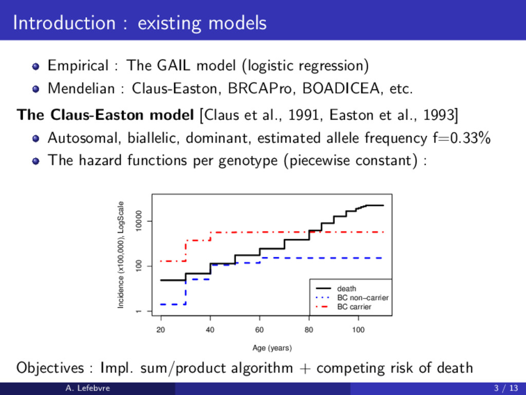
3. Introduction : existing models Empirical : The GAIL model (logistic regression) Mendelian : Claus-Easton, BRCAPro, BOADICEA, etc. The Claus-Easton model [Claus et al., 1991, Easton et al., 1993] Autosomal, biallelic, dominant, estimated allele frequency f=0.33% The hazard functions per genotype (piecewise constant) : 20 40 60 80 100 1 100 10000 Age (years) Incidence (x100,000), LogScale death BC non−carrier BC carrier Objectives : Impl. sum/product algorithm + competing risk of death A. Lefebvre 3 / 13
4. The model : the likelihood and the genotypes P (X, FH) = i P Xi |Xpati , Xmati genotypes × i P (PHi |Xi ) phenotypes , FH = {PHi }i Mode of inheritance : 1 autosomal biallelic gene, f = 0.33% Founders (Hardy-Weinberg ) :    P(Xi = 00) = (1 − f )2 P(Xi = 10) = P(Xi = 01) = f (1 − f ) P(Xi = 11) = f 2 Offsprings (Mendel):        P(Xi = 00) = (1 − Θ(Xpat)) × (1 − Θ(Xmat)) P(Xi = 10) = Θ(Xpat) × (1 − Θ(Xmat)) P(Xi = 01) = (1 − Θ(Xpat)) × Θ(Xmat) P(Xi = 11) = Θ(Xpat) × Θ(Xmat) with Θ(00) = 0, Θ(10) = Θ(01) = 0.5, Θ(11) = 1 A. Lefebvre 4 / 13
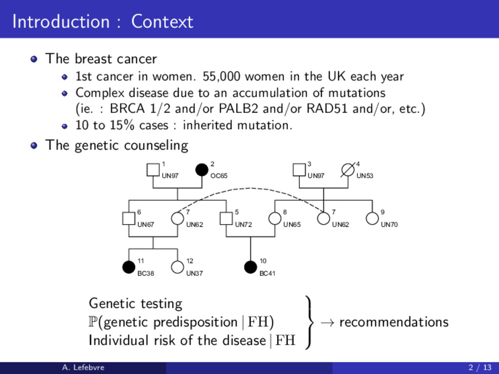
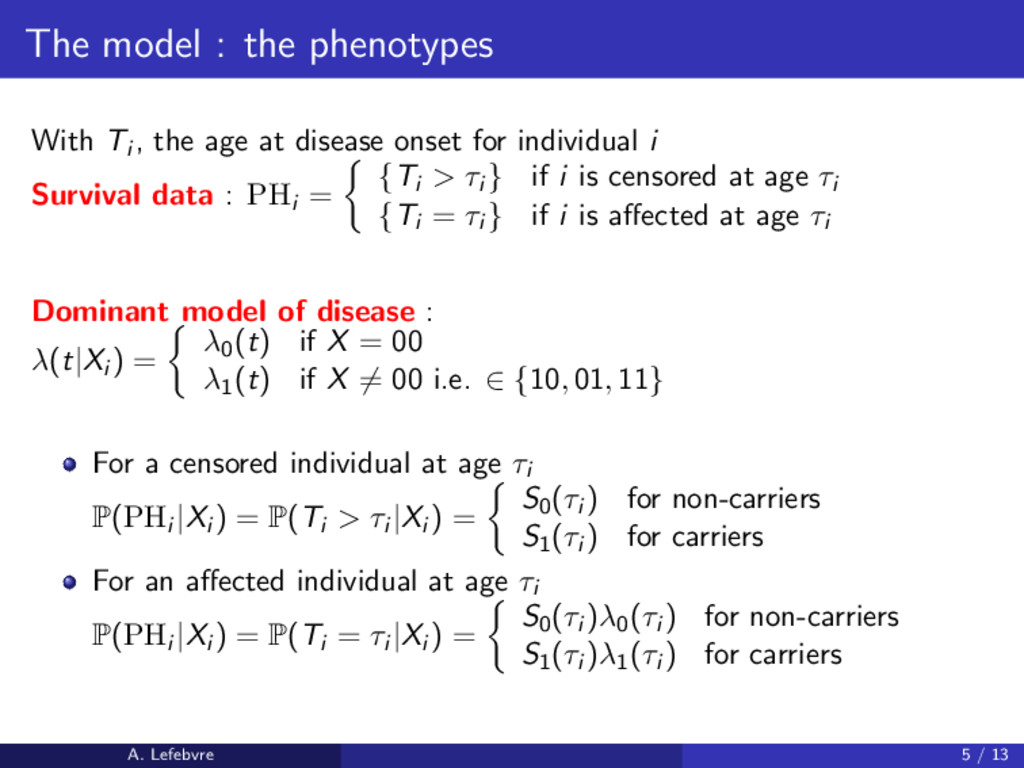
5. The model : the phenotypes With Ti , the age at disease onset for individual i Survival data : PHi = {Ti > τi } if i is censored at age τi {Ti = τi } if i is affected at age τi Dominant model of disease : λ(t|Xi ) = λ0(t) if X = 00 λ1(t) if X = 00 i.e. ∈ {10, 01, 11} For a censored individual at age τi P(PHi |Xi ) = P(Ti > τi |Xi ) = S0(τi ) for non-carriers S1(τi ) for carriers For an affected individual at age τi P(PHi |Xi ) = P(Ti = τi |Xi ) = S0(τi )λ0(τi ) for non-carriers S1(τi )λ1(τi ) for carriers A. Lefebvre 5 / 13
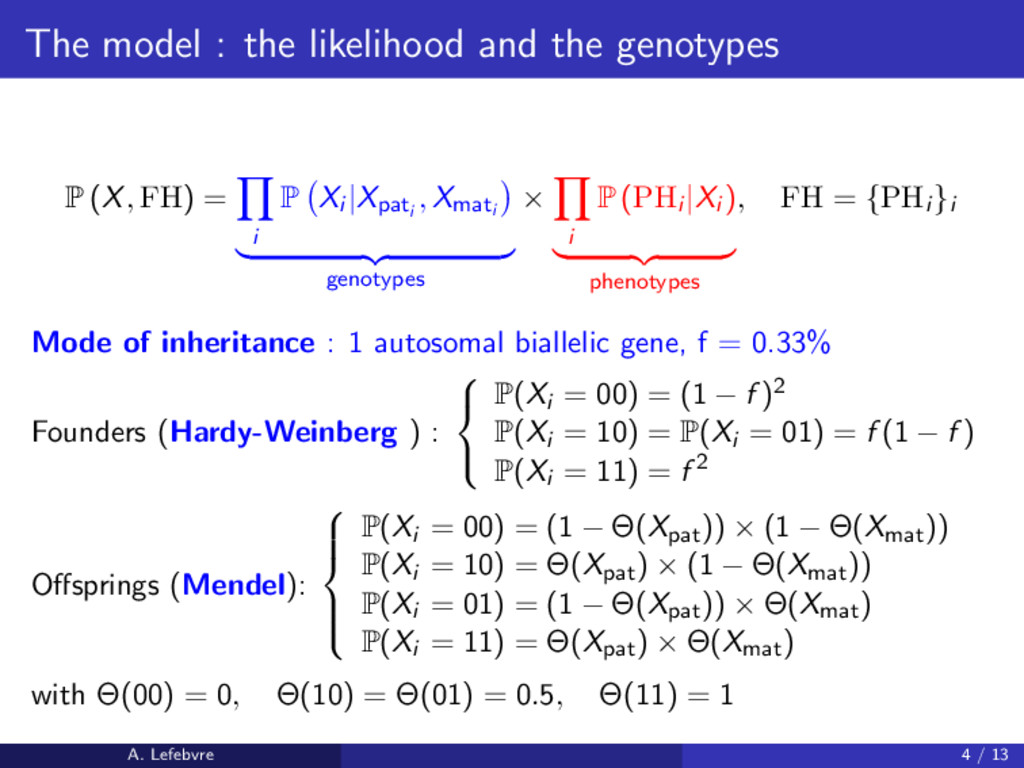
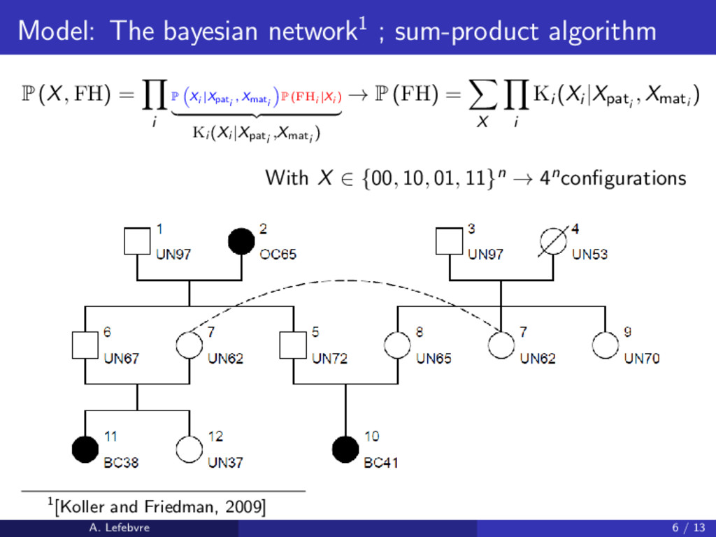
6. Model: The bayesian network1 ; sum-product algorithm P (X, FH) = i P Xi |Xpati , Xmati P (FHi |Xi ) Ki (Xi |Xpati ,Xmati ) → P (FH) = X i Ki (Xi |Xpati , Xmati ) With X ∈ {00, 10, 01, 11}n → 4nconfigurations 1[Koller and Friedman, 2009] A. Lefebvre 6 / 13
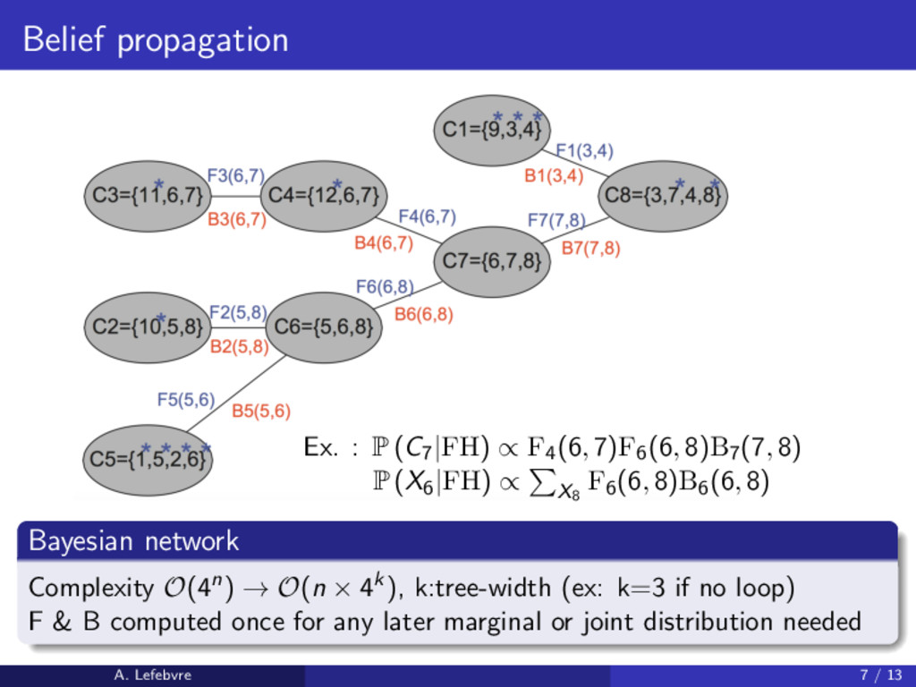
7. Belief propagation Ex. : P (C7|FH) ∝ F4(6, 7)F6(6, 8)B7(7, 8) P (X6|FH) ∝ X8 F6(6, 8)B6(6, 8) Bayesian network Complexity O(4n) → O(n × 4k), k:tree-width (ex: k=3 if no loop) F & B computed once for any later marginal or joint distribution needed A. Lefebvre 7 / 13
8. Model : Disease risk prediction for an unaffected individual π(τ) = P(carrier|FH) Breast cancer specific, no competing risk S(t|FH) = Xi P(T > t, Xi |FH) = π(τ) S1(t) S1(τ) + (1 − π(τ)) S0(t) S0(τ) π(t|FH) = π(τ)S1(t) S(t|FH)S1(τ) λdisease(t|FH) = π(t|FH)λ1(t) + (1 − π(t|FH))λ0(t) With competing risk of death : T∗ = min(Tdisease, Tdeath) λboth(t|FH) = λdisease(t|FH) + λdeath(t) : hazard function of T∗ P(T ≤ t|FH) = t τ Sboth(u)λdisease(u)du = t τ exp − u τ λboth(v)dv λdisease(u)du → discretized λ → closed form formulas for pch A. Lefebvre 8 / 13
9. Results : Carrier risk, posterior marginal carrier distribution 1 2 3 4 5 6 FH1 0.0 0.2 0.4 0.6 0.8 1.0 1 2 3 4 5 6 FH3 0.0 0.2 0.4 0.6 0.8 1.0 22/05/2017 11(17 Test 1 2 5 3 4 6 Test 1 2 OC51 5 3 UN61 4 6 A. Lefebvre 9 / 13
10. Results : Carrier risk, posterior marginal carrier distribution 1 2 3 4 5 6 FH4 0.0 0.2 0.4 0.6 0.8 1.0 1 2 3 4 5 6 FH5 0.0 0.2 0.4 0.6 0.8 1.0 22/05/2017 11(24 Test 1 2 OC51 5 3 UN61 4 6 BC29 *+,- 1 2 OC51 5 BC85 3 UN61 4 6 BC29 72 A. Lefebvre 10 / 13
11. Results, Disease risk, With competing death Test 1 UN97 2 OC65 3 UN97 4 UN53 6 UN67 7 UN62 5 UN72 8 UN65 7 UN62 9 UN70 11 BC38 12 UN37 10 BC41 A. Lefebvre 11 / 13
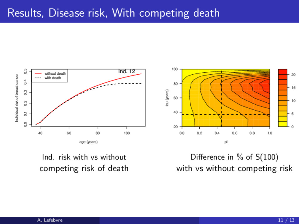
12. Results, Disease risk, With competing death 40 60 80 100 0.0 0.1 0.2 0.3 0.4 0.5 age (years) Individual risk of breast cancer Ind. 12 without death with death 0 5 10 15 20 0.0 0.2 0.4 0.6 0.8 1.0 20 40 60 80 100 pi tau (years) Ind. risk with vs without Difference in % of S(100) competing risk of death with vs without competing risk A. Lefebvre 11 / 13
13. Conclusion The model Adaptable (any genetic disease and model of disease) Fast (bayesian network - sum-product algorithm - belief propagation) Takes into account the competing risk of death What’s next? Parameters estimations Complex distributions (number of carriers in the family) with generating functions of probabilities (polynomials) → familial risk Multi-state and fragility models A. Lefebvre 12 / 13
14. Claus, E. B., Risch, N., and Thompson, W. D. (1991). Genetic analysis of breast cancer in the cancer and steroid hormone study. American journal of human genetics, 48(2):232. Easton, D., Bishop, D., Ford, D., and Crockford, G. (1993). Genetic linkage analysis in familial breast and ovarian cancer: results from 214 families. the breast cancer linkage consortium. American journal of human genetics, 52(4):678. Koller, D. and Friedman, N. (2009). Probabilistic graphical models: principles and techniques. MIT press. A. Lefebvre 13 / 13
15. Thank you for your attention A. Lefebvre 13 / 13