Statistical Analysis in Sports

Talk given to the Research, Evaluation, Measurement, and Statistics graduate seminar at the University of Kansas

Transcript

1. Statistical Analysis in Sports Jake Thompson
2. October 9, 2015 Statistical Analysis in Sports 2 Creating a Rating System § Measuring success in basketball § Possessions § Scoring efficiency § Turning statistics into a rating system § Expected winning percentages § Using the ratings § Predicting games § Predicting point spreads § Alternative rating methodologies § Elo § Correlated-Gaussian
3. Measuring Success in Basketball
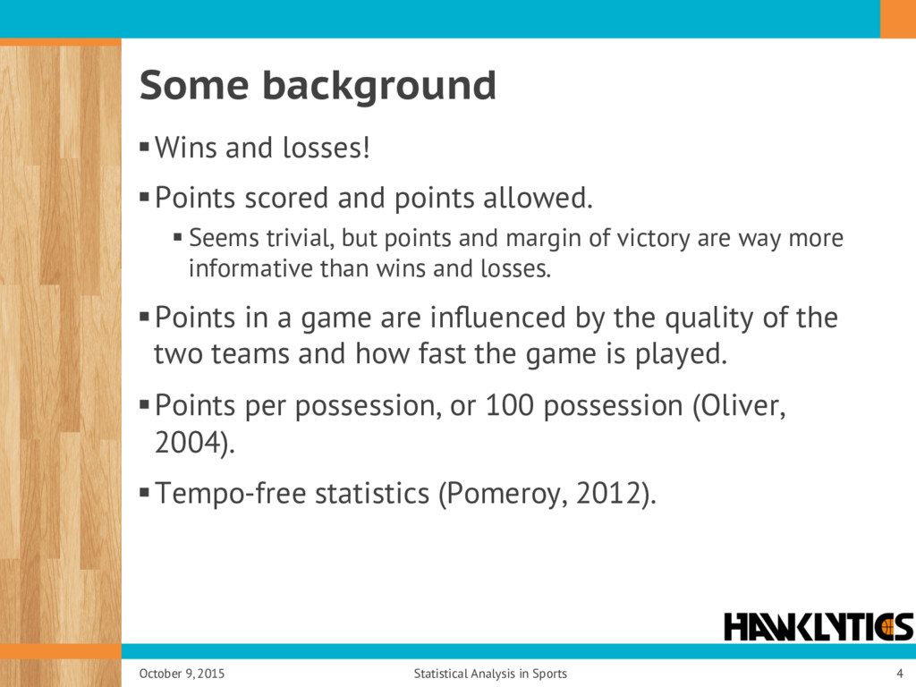
4. Some background § Wins and losses! § Points scored and points allowed. § Seems trivial, but points and margin of victory are way more informative than wins and losses. § Points in a game are influenced by the quality of the two teams and how fast the game is played. § Points per possession, or 100 possession (Oliver, 2004). § Tempo-free statistics (Pomeroy, 2012). October 9, 2015 Statistical Analysis in Sports 4
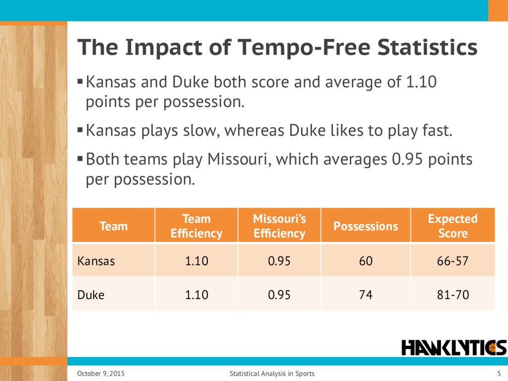
5. The Impact of Tempo-Free Statistics § Kansas and Duke both score and average of 1.10 points per possession. § Kansas plays slow, whereas Duke likes to play fast. § Both teams play Missouri, which averages 0.95 points per possession. October 9, 2015 Statistical Analysis in Sports 5 Team Team Efficiency Missouri’s Efficiency Possessions Expected Score Kansas 1.10 0.95 60 66-57 Duke 1.10 0.95 74 81-70
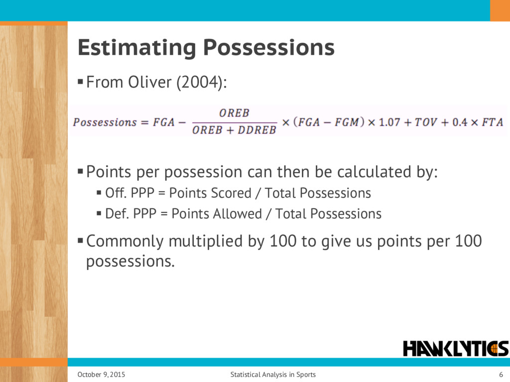
6. Estimating Possessions § From Oliver (2004): § Points per possession can then be calculated by: § Off. PPP = Points Scored / Total Possessions § Def. PPP = Points Allowed / Total Possessions § Commonly multiplied by 100 to give us points per 100 possessions. October 9, 2015 Statistical Analysis in Sports 6
7. Example: Kansas vs. Iowa State October 9, 2015 Statistical Analysis in Sports 7 Team Points FGM FGA OREB DREB TOV FTA Kansas 89 32 63 10 25 15 23 Iowa State 76 30 72 15 22 14 14
8. Adjusting for Strength of Schedule § Generalized Least Squares (gls in R). § PPP = OffenseT + DefenseO § KU PPP = OffenseKU + DefenseISU § PPP = β 0 + β Off + β Def + β Off_HC + β Def_HC § 117.43 = β 0 + β KU_Off + β ISU_Def + β Off_HC § 100.28 = β 0 + β ISU_Off + β KU_Def + β Def_HC § The gls() function in R allows us to correlate errors within a grouping variable. § Scores are nested within games. October 9, 2015 Statistical Analysis in Sports 8
9. Specifying the Model § The parameters: § One offensive parameter per team (350) § One defensive parameter per team (350) § One intercept § Two home court parameters § Selecting the reference teams § One reference on offense and defense § Selected iteratively § Originally the last team alphabetically § Model rerun with reference team set to the team with the average offensive/defensive efficiency. October 9, 2015 Statistical Analysis in Sports 9
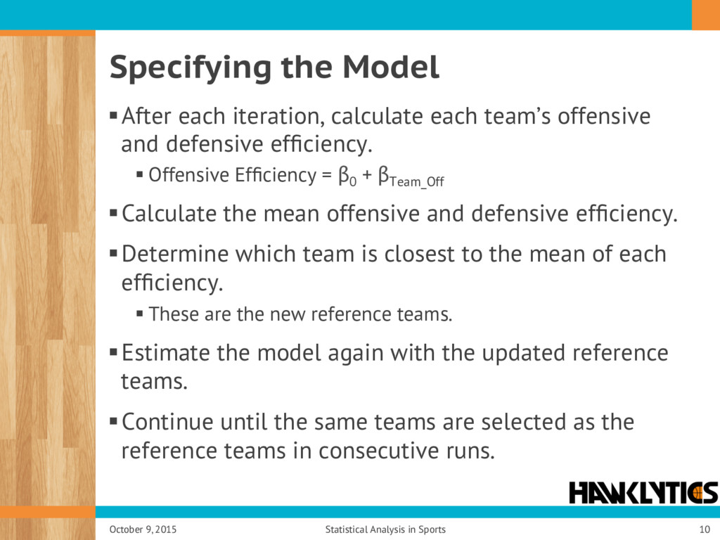
10. Specifying the Model § After each iteration, calculate each team’s offensive and defensive efficiency. § Offensive Efficiency = β 0 + β Team_Off § Calculate the mean offensive and defensive efficiency. § Determine which team is closest to the mean of each efficiency. § These are the new reference teams. § Estimate the model again with the updated reference teams. § Continue until the same teams are selected as the reference teams in consecutive runs. October 9, 2015 Statistical Analysis in Sports 10
11. Results October 9, 2015 Statistical Analysis in Sports 11 School Conference Offense Defense Net Kentucky SEC 120.21 78.51 41.70 Duke ACC 124.26 88.00 36.26 Wisconsin Big Ten 127.09 89.92 37.17 Arizona Pac-12 118.44 84.05 34.39 Villanova Big East 120.73 86.99 33.75 Virginia ACC 114.90 80.94 33.96 Gonzaga WCC 120.19 89.22 30.97 Utah Pac-12 116.14 85.55 30.59 North Carolina ACC 118.48 90.31 28.17 Ohio State Big Ten 115.50 89.39 26.11 Notre Dame ACC 123.85 96.89 26.96 Oklahoma Big 12 110.34 84.68 25.66 Kansas Big 12 114.19 88.57 25.62 Louisville ACC 108.44 83.98 24.47 Iowa State Big 12 117.07 92.66 24.41
12. Turning Statistics Into a Rating System
13. Expected Winning Percentage § Pythagorean Win Expectation (James, 1983) § If teams win in proportion to their “quality”, n = 2. § n varies by sport, and reflects the role that chance plays in the outcome of games. § MLB: n = 1.83 § NHL: n = 2.15 § NFL: n = 2.37 § NBA: n = 16.5 October 9, 2015 Statistical Analysis in Sports 13
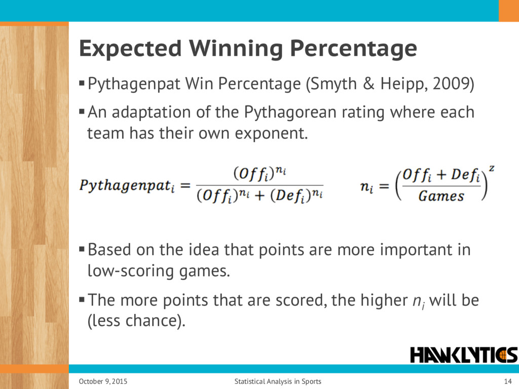
14. Expected Winning Percentage § Pythagenpat Win Percentage (Smyth & Heipp, 2009) § An adaptation of the Pythagorean rating where each team has their own exponent. § Based on the idea that points are more important in low-scoring games. § The more points that are scored, the higher ni will be (less chance). October 9, 2015 Statistical Analysis in Sports 14
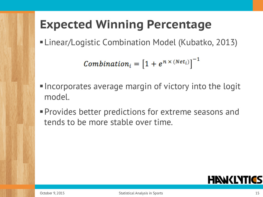
15. Expected Winning Percentage § Linear/Logistic Combination Model (Kubatko, 2013) § Incorporates average margin of victory into the logit model. § Provides better predictions for extreme seasons and tends to be more stable over time. October 9, 2015 Statistical Analysis in Sports 15
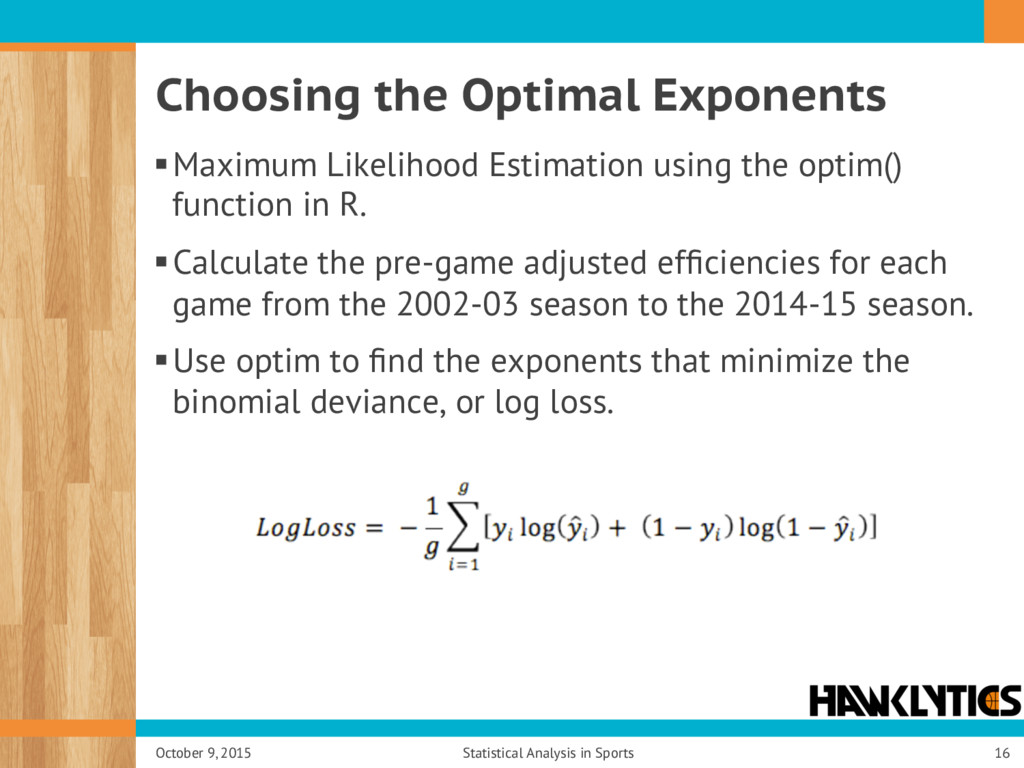
16. Choosing the Optimal Exponents § Maximum Likelihood Estimation using the optim() function in R. § Calculate the pre-game adjusted efficiencies for each game from the 2002-03 season to the 2014-15 season. § Use optim to find the exponents that minimize the binomial deviance, or log loss. October 9, 2015 Statistical Analysis in Sports 16
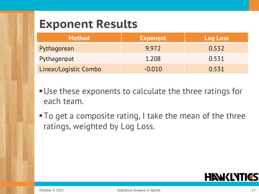
17. Exponent Results § Use these exponents to calculate the three ratings for each team. § To get a composite rating, I take the mean of the three ratings, weighted by Log Loss. October 9, 2015 Statistical Analysis in Sports 17 Method Exponent Log Loss Pythagorean 9.972 0.532 Pythagenpat 1.208 0.531 Linear/Logistic Combo -0.010 0.531
18. Team Rating Results October 9, 2015 Statistical Analysis in Sports 18 School Conf. Pythagorean Pythagenpat Linear/ Logistic Composite Kentucky SEC 0.9859 0.9850 0.9846 0.9851 Wisconsin Big Ten 0.9692 0.9776 0.9760 0.9743 Duke ACC 0.9690 0.9751 0.9738 0.9726 Arizona Pac-12 0.9683 0.9691 0.9686 0.9687 Virginia ACC 0.9705 0.9670 0.9672 0.9682 Villanova Big East 0.9634 0.9676 0.9665 0.9658 Gonzaga WCC 0.9513 0.9576 0.9563 0.9551 Utah Pac-12 0.9547 0.9550 0.9547 0.9548 North Carolina ACC 0.9375 0.9442 0.9431 0.9416 Notre Dame ACC 0.9204 0.9391 0.9362 0.9319 Ohio State Big Ten 0.9279 0.9315 0.9310 0.9302 Oklahoma Big 12 0.9334 0.9269 0.9281 0.9294 Kansas Big 12 0.9265 0.9280 0.9278 0.9274 Baylor Big 12 0.9237 0.9253 0.9251 0.9247 Louisville ACC 0.9276 0.9179 0.9197 0.9217
19. Using the Ratings
20. Predicting Game Winners § We can calculate a team’s probability of beating their opponent by using the Log5 formula (James, 1981). § This model generalizes to include the Bradley-Terry-Luce model commonly used in psychology, and the Rasch model in psychometrics (Long, 2013). § Kansas (0.9274) vs. Ohio State (0.9302): October 9, 2015 Statistical Analysis in Sports 20
21. Calculating Point Spreads § From the GLS model: § PS = (β 0 + β T1_Off + β T2_Def ) - (β 0 + β T2_Off + β T1_Def ) § Directly from the adjusted efficiencies: § Team 1 Points = (T1Off / υ Off ) × (T2Def / υ Def ) × υ All § Team 2 Points = (T2Off / υ Off ) × (T1Def / υ Def ) × υ All § PS = Team 1 Points – Team 2 Points § From net ratings: § PS = (T1Off – T1Def ) – (T2Off – T2Def ) October 9, 2015 Statistical Analysis in Sports 21
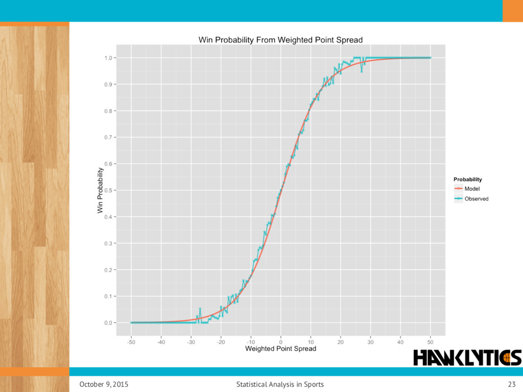
22. Calculating a Weighted Point Spread § For each point spread method, compare the projected point spread to the actual margin of victory: § Calculate expected point spread for each game by averaging the three methods, weighted by RMSE. § We can also calculate win probabilities from the projected point spreads using logistic regression. October 9, 2015 Statistical Analysis in Sports 22 Method RMSE Weight GLS 10.774 0.331 Average Efficiencies 10.664 0.334 Net Efficiencies 10.651 0.335
23. October 9, 2015 Statistical Analysis in Sports 23
24. October 9, 2015 Statistical Analysis in Sports 24
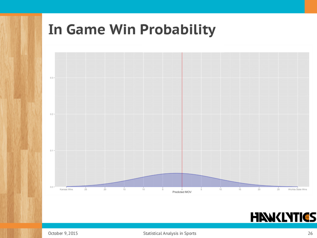
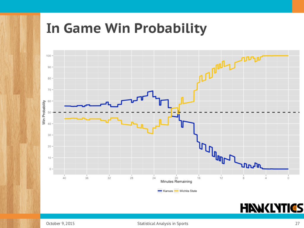
25. In Game Win Probability § Adapted and expanded from Winston (2012) and Paine (2012). § Model assumes the margin of victory of a given game is ~N(PS, 10.612). § The mean and standard deviation of the distribution over the course of a game are given by: § StDev = 10.612 / sqrt(40 / minutes remaining) § Mean = (PS * (minutes remaining / 40)) + (Margin * (40 / minutes played)) § The win probability is given by the proportion of the distribution covering margins of victory that would result in the team winning. October 9, 2015 Statistical Analysis in Sports 25
26. In Game Win Probability October 9, 2015 Statistical Analysis in Sports 26
27. In Game Win Probability October 9, 2015 Statistical Analysis in Sports 27
28. Alternate Rating Methods
29. Elo Ratings § Named after physics professor Arpad Elo. § Most widely used in chess and international soccer. § How it works: § Given a starting state of two teams, how is each team expected to perform? § How did the teams actually perform? § Update the ratings with this new information. October 9, 2015 Statistical Analysis in Sports 29
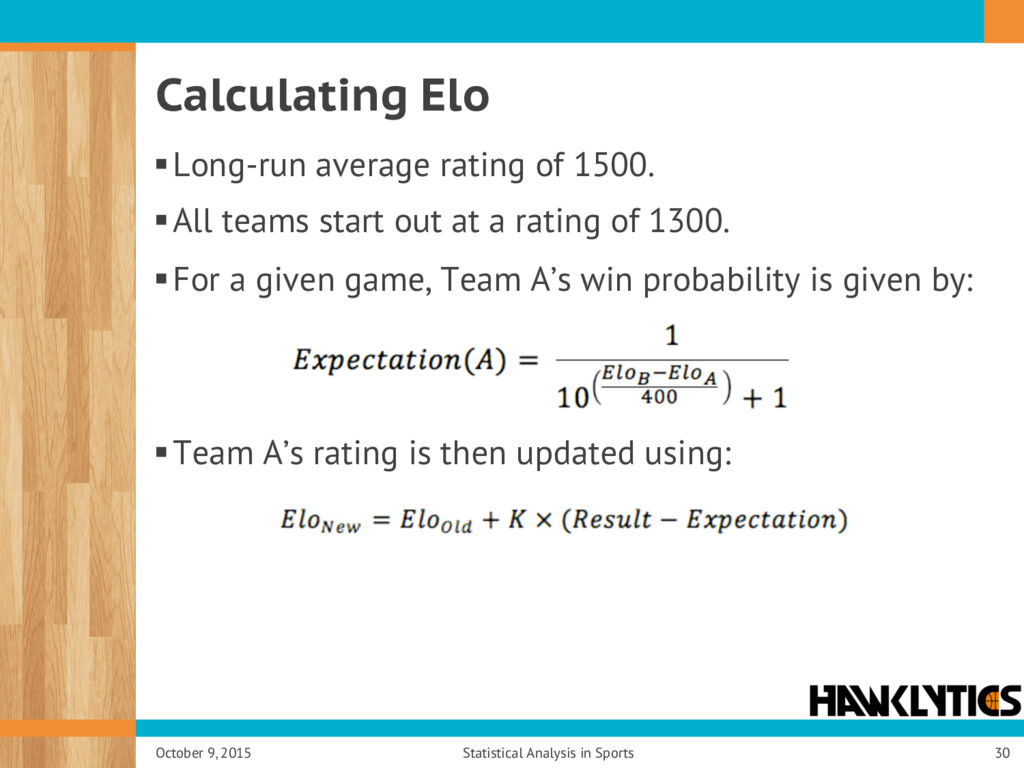
30. Calculating Elo § Long-run average rating of 1500. § All teams start out at a rating of 1300. § For a given game, Team A’s win probability is given by: § Team A’s rating is then updated using: October 9, 2015 Statistical Analysis in Sports 30
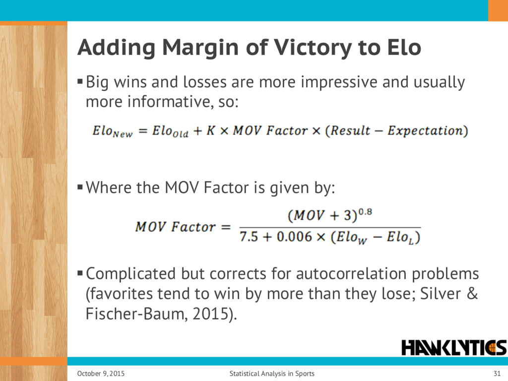
31. Adding Margin of Victory to Elo § Big wins and losses are more impressive and usually more informative, so: § Where the MOV Factor is given by: § Complicated but corrects for autocorrelation problems (favorites tend to win by more than they lose; Silver & Fischer-Baum, 2015). October 9, 2015 Statistical Analysis in Sports 31
32. Elo Ratings Pros/Cons § Pros: § Easy to calculate § Only need game scores (location can also be added in) § Track historical trends § Cons: § Ratings heavily dependent on performance in previous seasons (can be less accurate early in season) § Ratings are not retroactively adjusted to account for team’s being better/worst than expected. October 9, 2015 Statistical Analysis in Sports 32
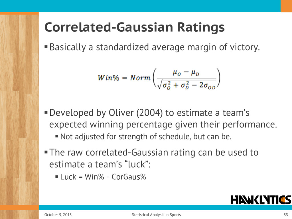
33. Correlated-Gaussian Ratings § Basically a standardized average margin of victory. § Developed by Oliver (2004) to estimate a team’s expected winning percentage given their performance. § Not adjusted for strength of schedule, but can be. § The raw correlated-Gaussian rating can be used to estimate a team’s “luck”: § Luck = Win% - CorGaus% October 9, 2015 Statistical Analysis in Sports 33
34. References James, B. (1981). Baseball Abstracts. Lawrence, KS: Privately Printed. James, B. (1983). Baseball Abstracts. New York: Ballantine Books. Kubatko, J. (2013). Pythagoras of the hardwood [Web log post]. Retrieved from http://statitudes.com/blog/ 2013/09/09/pythagoras-of-the-hardwood/ Long, C. (2013). Baseball, chess, psychology, and psychometrics: Everyone uses the same damn rating system [Web log post]. Retrieved from http://angrystatistician.blogspot.com/2013/03/baseball-chess- psychology-and.html Oliver, D. (2004). Basketball on paper: Rules and tools for performance analysis. Dulles, Virginia: Potomac Books, Inc. Paine, N. (2012). Are NFL playoff outcomes getting more random? [Web log post]. Retrieved from http:// www.footballperspective.com/are-nfl-playoff-outcomes-getting-more-random/ Pomeroy, K. (2012, June 8). Ratings glossary [Web log post]. Retrieved from http://kenpom.com/blog/index.php/ weblog/entry/ratings_glossary Silver, N. & Fischer-Baum, R. (2015). How we calculate NBA Elo ratings [Web log post]. Retrieved from http:// fivethirtyeight.com/features/how-we-calculate-nba-elo-ratings/ Smyth, D. & Heipp, B. (2009). Runs Per Win From Pythagenpat [Web log post]. Retrieved from http:// walksaber.blogspot.com/2009/01/runs-per-win-from-pythagenpat.html Winston, W. (2012). Mathletics: How gamblers, managers, and sports enthusiasts use mathematics in baseball, basketball, and football. Princeton, NJ: Princeton University Press. October 9, 2015 Statistical Analysis in Sports 34