Separation of bounded arithmetics using a consistency statement

Transcript

1. Separation of bounded arithmetic using a consistency statement Yoriyuki Yamagata AIST, Japan Sep. 1, 2019
2. This presentation about ... A possible proof strategy of Separation of Buss’s S1 2 and S2, S1 2 S2 (?) As a corollary, P = NP (?!) I do not believe it at all, but it may contain interesting techniques or conjectures Draft: https://www.dropbox.com/s/g22x84rfdqmyx82/
3. Draft Location
4. Definition of Buss’s Si 2 Si 2 is formulated by PIND for Σb i -formula plus axioms Ax. 1 Ax is finite, 2 all formulas in Ax are true in the standard interpretation, 3 all formulas in Ax is quantifier free, 4 Ax implies all BASICe axioms in [Buss and Ignjatovi´ c, 1995] 5 Ax implies formulas corresponding P = NP in [Takeuti, 1996] if P = NP. S2 := i=1,2,... Si 2
5. Definition of Cook and Urquhart’s PV Defining axioms for polynomial-time functions Identity axioms Substitution axiom Induction axiom PV− is a system obtained from PV by dropping induction axiom PV− 1 = PV− + first order logic PV− 1 (D) is the restriction of PV− 1 in which the number of quantifiers and equations is bounded by D.
6. Proof strategies 1 Define PV− q (D), an extension of PV− with finite number D of Henkin-like quantifiers 2 Prove consistency of PV− q (D) in S2 3 Embed PV− 1 (D) to PV− 1 (D) in S2 4 Prove embedded PV− 1 (D) + Ax is consistent in S2 5 Prove consistency of PV− 1 (D) + Ax is not provable in S1 2 5. is modification of [Buss and Ignjatovi´ c, 1995] Our tasks are 1-4
7. Dependency matrix Definition A dependency matrix Q is a sequence of 1 x(x1, . . . , xn) 2 {x}(x1, . . . , xn) in which all x are different (but x1, . . . , xn may have overlap) x(x1, . . . , xn) is a existential quantification which depends on x1, . . . , xn {x}(x1, . . . , xn) is a universal quantification which depends on x1, . . . , xn A dependency matrix is almost like a Henkin quantifier [Krynicki and Mostowski, 1995], but the order has meaning (to construct a semantics)
8. Language and proofs of PV− q (D) Definition Language of S2 plus Boolean variables and terms Additional functions bit(x, y): |y|-th bit of x p is the if-then-else function p(⊥, x, y) = x and p( , x, y) = y Boolean functions !, &, ||, →, ↔ A formula of PV− q is a form Q =⇒ φ where Q is a dependency matrix and φ is an equation Definition PV− q (D)-proofs are tree of PV− q (D)-formulas built by the following axioms and rules
9. Axioms All defining axioms for polynomial-time functions plus bit(ε, xW) = ⊥ bit(0xW, ε) = ⊥ bit(1xW, ε) = bit(bx, b y) = bit(x, y) p(⊥, x, y) = x p( , x, y) = y Finite many axioms of Boolean algebra t(x1, . . . , xn) = u(x1, . . . , xn)
10. Inference: quantifier reordering Q1, x(x), y([x, ]y), Q2 =⇒ φ Q1, y([x, ]y), x(x), Q2 =⇒ φ Q1, {x}(x), {y}([x, ]y), Q2 =⇒ φ Q1, {y}([x, ]y), {x}(x), Q2 =⇒ φ Q1, x(x), {y}(y), Q2 =⇒ φ Q1, {y}(y), x(x), Q2 =⇒ φ Q1, {x}(x), y(y), Q2 =⇒ φ Q1, y(y), {x}(x), Q2 =⇒ φ where y ∈ {x} and x ∈ {y} and [. . .] means it is optional
11. Inference: removing unused quantification Q1, x(y), Q2 =⇒ φ Q1, Q2 =⇒ φ Q1, {x}(y), Q2 =⇒ φ Q1, Q2 =⇒ φ if x is not a free variable in Q2 =⇒ φ
12. Inference: introduction and elimination of quantifiers Q =⇒ φ(y) {y}(y), Q =⇒ φ(y) Q =⇒ φ(t) Q, x(FV(t)) =⇒ φ(x) if y is not a bound variable of Q and y is a free variables of Q =⇒ φ(y) Q1, {x}(x) =⇒ φ(x) Q1 =⇒ φ(t) if FV(t) ⊆ {x}
13. Inference: axioms and equality rules Q1 =⇒ φ for axiom φ Q1 =⇒ u = t Q1 =⇒ t = u Q1 =⇒ t = u Q2 =⇒ u = r Q1, Q2 =⇒ t = r u if Q1, Q2 is a well-formed dependency matrix
14. Inference: compatibility of equality and p-rule Q1 =⇒ t1 = u1 · · · Qn =⇒ tn = un Q1, . . . , Qn =⇒ f (t1, . . . , tn) = f (u1, . . . , un) Q1 =⇒ t1 = u1 Q2 =⇒ t2 = u2 Q1, Q2 =⇒ p(b, t1, t2) = p(b, u1, u2)
15. A computation: idea A PV− q -proof of . . . . Q =⇒ t = u is interpreted as a constraction of a “computation” of ξ(u) from a “computation” of ξ(t) and reverse direction, where quantifiers Q is interpreted by substitutions ξ
16. A computation: problem I Problem I The size of a computation can be exponential, e.g. 2#2#2# · · · #2 Therefore, the proof cannot construct a computation of the lefthand from the righthand proj1 2 (0, 2#2#2# · · · #2) = 0 Solution Introduce unknown value ∗
17. A computation: problem II Problem What is the value of bit(∗, ∗)? We want to interpret the value of a Boolean term as a real Boolean, not, for example, a three-valued logic, so that we can prove that ⊥ = is never derived Solution We choose the value of bit(∗, ∗) randomly, yet consistently across the same computation. For this purpose, we incorporate the evaluation of bit(∗, ∗) into an evaluation environment ρ
18. Approximate value: g-numerals Definition g-numerals v ∈ W := ε | ∗ | 0v | 1v Approximate relation is defined as: ε ε, v ∗, v w =⇒ bv bw for b = 0, 1, If v w then w is often written as v∗. G-numerals and Boolean values are called g-values
19. A environment and computation statement Definition An environment ρ of t is a map uW → v ∈ W uB → b ∈ B = {⊥, } for subformulas of t t ∈ dom(ρ) ⇐⇒ ρ(t) is defined. Definition A computational statement is a form t, ρ ↓ v where t is a term, ρ is an environment and v is a g-value.
20. Computation rules I Computations are DAGs built by the following rules: tW, ρ ↓ ∗ ∗ x, ρ ↓ v∗ Env where v = ρ(x) v, ρ ↓ v∗ v where v is a numeral t, ρ ↓ v bt, ρ+ ↓ bv∗ b where b is either 0 or 1 and t is not a numeral.
21. Computation rules II ( ti , ρ ↓ vi )i=1,...,m εm(t1, . . . , tm), ρ+ ↓ ε εm ( tj , ρ ↓ vj )j=1,...,m proji m (t1, . . . , tm), ρ+ ↓ v∗ i proji m t, ρ ↓ ⊥ u1, ρ ↓ v1 u2, ρ ↓ v2 p(⊥, u1, u2), ρ+ ↓ v∗ 1 p t, ρ ↓ u1, ρ ↓ v1 u2, ρ ↓ v2 p( , u1, u2), ρ+ ↓ v∗ 2 p
22. Computation rules III t, ρ ↓ v u, ρ ↓ w bit(t, u), ρ ↓ b bit where b is determined by bit(ε, w) = ⊥ if w = ∗ bit(bv, ε) = b bit(bv, b w) = bit(v, w). If bit(v, w) function is undefined, we often write bit(v, w) = ∗. If bit(v, w) = ∗, we put b = ρ(bit(t, u)).
23. Computation rules IV For Boolean connectives t, ρ ↓ b !t, ρ ↓ !b ! t1, ρ ↓ b1 t2, ρ ↓ b2 t1&t2, ρ ↓ b1&b2 & ⊥, ρ ↓ ⊥ ⊥ , ρ ↓ If f is defined by composition, we have the following rule. g(y, ξ ↓ z h1(x), ν ↓ w1 · · · hm(x), ν ↓ wm ( ti , ρ ↓ vi )i=1,...,n f (t1, . . . , tn), ρ+ ↓ z∗ where y = y1, . . . , ym, x = x1, . . . , xn, ν(xi ) = vi , i = 1, . . . , n and ξ(yj ) = wj , j = 1, . . . , m.
24. Computation rules V If f is defined by recursion, we have the following rules. gε(x1, . . . , xn), ξ ↓ z t, ρ ↓ ε ( ti , ρ ↓ vi )i=1,...,n f (t, t1, . . . , tn), ρ+ ↓ z∗ rec-ε where ξ(xi ) = vi for i = 1, . . . , n. gb(x0, y, x), ξ ↓ z t, ρ ↓ bv0 f (x0, x), ν ↓ w ( tj , ρ ↓ vj )j=1,...,n f (t, t1, . . . , tn), ρ+ ↓ z∗ where b = 0, 1 and x = x1, . . . , xn. The environment ν is defined by ν(xj ) = vj for j = 1, . . . , n and ν(x0) = v0 while ξ is defined by ξ(xj ) = vj , ξ(x0) = v0, ξ(y) = w.
25. Complexity of computations Definition For a computation σ, C(σ) is the minimum value which satisfies nodes(σ) ≤ C(σ) size(t) ≤ C(σ) if t, ρ ↓ v ∈ σ nodes(v) ≤ C(σ) if t, ρ ↓ v ∈ σ
26. Basic properties - computation of successors Lemma (S1 2 ) If ε, ρ ↓ v is contained in a computation σ, then either v ≡ ε or v ≡ ∗. If bt, ρ ↓ v where t is not a numeral, is contained in σ, then either v ≡ bv0 for some g-value v0 or v ≡ ∗. If v ≡ bv0, then σ contains t, ρ∗ ↓ v0 and v0 v0. Proof. Induction on σ
27. Basic properties - computation of numerals Lemma (S1 2 ) If v, ρ ↓ w, in which v are a numeral, is contained in a computation σ, then v w. Proof. Only rules which can derive v, ρ ↓ w are ∗ and v-rules.
28. Maximal environment Definition (maximal environment) For an environment ρ and a term of type W, we define V (t, ρ) = {v | σ t, ρ ↓ v, C(σ) ≤ nodes(t) · U} vals(t, ρ) = {v ∈ V (t, ρ) | v ∈ V (t, ρ), v v =⇒ v = v} ρ is maximal if ρ(t) ∈ vals(t, ξ) and ρ(bit(a, b)) = bit(ρ(a), ρ(b)) if bit(ρ(a), ρ(b)) = ∗. Env(ρ, t, U) ⇐⇒ ρ is a maximal environment . Env(ρ, t, U) is a bounded formula.
29. Substitution into ρ Lemma Let ρ be a maximal environment. Then, there is a maximal environment ρ such that ρ (x) = ρ(u) ρ(t(u)) ρ (t(x))
30. Basic properties - compatibility lemma Definition is defined as v w ⇐⇒ either v w or w v ρ1 ρ2 ⇐⇒ ρ1(t) ρ2(t) for any t ∈ dom(ρ1) ∩ dom(ρ2) For Boolean b1, b2, define b1 b2 ⇐⇒ b1 = b2 Lemma (S2: Compatibility lemma) Let ρ1 and ρ2 be maximal environments which satisfy ρ1 ρ2, t be the term. If both of t, ρ1 ↓ v and t, ρ2 ↓ w are contained in computations σ and τ respectively, then v w.
31. Most accurate evaluation in σ Definition Compatibility lemma allows extracting the most “accurate” value v(t, ρ, σ) of t evaluated in a maximal environment ρ from a computation
32. Basic properties - substitution lemma I Lemma (S2, Substitution Lemma I) Let ρ be a maximal environment and σ be a computation with conclusions t1(u1, . . . , un), ρ ↓ v1, . . . , tm(u1, . . . , un), ρ ↓ vm. Let ρ be the maximal environment which extends ρ by ρ (xi ) = v(ui , ρ, σ) and ρ (bit(a(x), b(x))) = ρ(bit(a(u), b(u))). Then, there is a computation τ with conclusions t1(x), ρ ↓ v1, . . . , tm(x), ρ ↓ vm. such that C(τ) ∈ C(σ) + m j=1 size(tj (ε, . . . , ε))
33. Basic properties - substitution lemma II Lemma (S2, Substitution Lemma II) Let ρ be a maximal environment and ρ is the maximal extension of ρ such that ρ (xi ) = wi and ρ (bit(r(x), s(x))) = ρ(bit(r(u), s(u))). Assume that size(tj (u1, . . . , un)) ≤ C, j = 1, . . . , m. Then for any computation σ with conclusions tj (x1, . . . , xn), ρ ↓ vj for j = 1, . . . , m such that ρ(xi ) = v(ui , ρ, σ), there is a computation τ such that τ has all conclusions of σ plus tj (u1, . . . , un), ρ ↓ vj for j = 1, . . . , m as conclusions and C(τ) ≤ max(C(σ) + m j=1 size(tj (ε, . . . , ε)), C).
34. Basic properties - defining axiom I Lemma (S2, defining axiom I) Let f (u(r)) = t(r) is a substitution instance of the defining axiom f (u(y)) = t(y). Let ρ be a maximal environment and α judgements. If σ is a computation of f (u(r)), ρ ↓ v, α, there is a computation τ of t(r), ρ ↓ v, α such that C(τ) ≤ C(σ) + size(f (u(r)) = t(r)) Further, τ derives α from the same assumptions using the same rule to σ.
35. Basic properties - defining axiom II Lemma (S2, defining axiom II) Let f (u(r)) = t(r) is a substitution instance of the defining axiom f (u(y)) = t(y). Let ρ be a maximal environment and α judgements. If σ is a computation of t(r), ρ ↓ v, α, there is a computation τ of f (u(r)), ρ ↓ v, α such that C(τ) ≤ C(σ) + size(f (u(r)) = t(r)) Further, τ derives α from the same assumptions using the same rule to σ.
36. Basic properties - Boolean axioms Lemma (S2, Boolean axioms) Let t(r) = u(r) (1) a substitution instance of a valid Boolean axiom t(y) = u(y). Let ρ be a maximal environment and α judgements. If σ is a computation of t(r), ρ ↓ b, α, there is a computation τ of u(r), ρ ↓ b, α such that C(τ) ≤ C(σ) + size(t(r) = u(r)) (2)
37. Consistency proof - preliminaries Definition [q1/x1] · · · [qd /xd ], d ≤ D is called substitution sequence if x1, . . . , xd are all different dom(ξ) = {x1, . . . , xd } ξ(t) ≡ t[qd /xd ] · · · [q1/x1] B(ξ) = max{size(ξ(xi )) | i = 1, . . . , d} ξ : η is the concatenation of ξ and η Env(ρ, t, U): ρ is a maximal environment or t. U is the same U in the definittion of maximal environments.
38. Consistency proof - Sat relation for equality Definition U, B be integers such that U ≥ 2B ρ a maximal environment α judgements ξ be a substitution sequence such that B(ξ) ≤ (U − B)d Sat(U, B, ξ, ρ, α, t = u) ⇐⇒ ∀σ ξ(t), ρ ↓ v, α s.t. C(σ) ≤ (U − B)D+2, ∃τ ξ(u), ρ ↓ v, α s.t. C(τ) ≤ C(σ) + BD+2 and ∀τ ξ(u), ρ ↓ v, α s.t. C(τ) ≤ (U − B)D+2, ∃σ ξ(t), ρ ↓ v, α s.t. C(σ) ≤ C(τ) + BD+2
39. Consistency proof - Sat relation for quantifiers Definition For universal, Sat(U, B, ξ, ρ, α, {x}(z1, . . . , zm), Γ =⇒ φ) ⇐⇒ ∀q, B([q/x] : ξ) ≤ (U − B)d , s.t. FV(q) ⊆ {z1, . . . , zm}, Sat(U, B, [q/x] : ξ, ρ, α, Γ =⇒ φ) For existential, Sat(U, B, ξ, ρ, α, x(z1, . . . , zm), Γ =⇒ φ) ⇐⇒ B ≤ ∀B ≤ U/2, ∃q, B([q/x] : ξ) ≤ (U − B )d s.t. FV(q) ⊆ {z1, . . . , zm}, Sat(U, B , [q/x] : ξ, ρ, α, Γ =⇒ φ)
40. Consistency proof - properties of Sat Lemma (S2, monotonicity) If B1 ≤ B2, Sat(U, B1, ξ, ρ, α, S) =⇒ Sat(U, B2, ξ, ρ, α, S) Lemma (S2, substitution for Sat) Let p be a term such that ξ(q) = q. ∀ρ, Env(ρ, t(x), UD+2) ∧ Env(ρ, u(x), UD+2) → Sat(U, B, ξ, ρ, α, t(x) = u(x)) =⇒ ∀ρ, Env(ρ, t(q), UD+2) ∧ Env(ρ, u(p), UD+2) → Sat(U, B + size(t(ε) = u(ε)), ξ, ρ, α, t(q) = u(q))
41. Consistency proof - soundness theorem Theorem (S2, soundness) a proof χ of PV− q (D) of S ≡ Q =⇒ φ an integer U s.t. U ≥ 2size(χ) a substitution sequence η ≡ [q1/x1] · · · [qd /xd ] s.t. B(η) ≤ (U − size(χ))d a sequence of statements α s.t. M(α) ≤ (U − size(χ))D+2 where M(α) is the maximum size of terms appearing in α. Then, Sat(U, size(χ), η, ρ, α, S) holds.
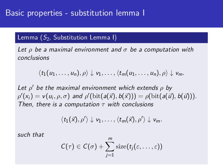
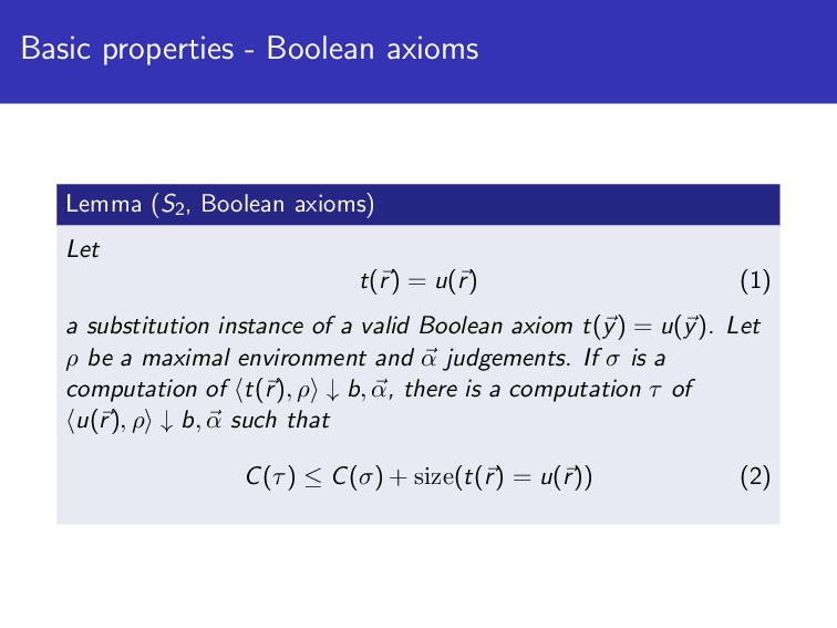
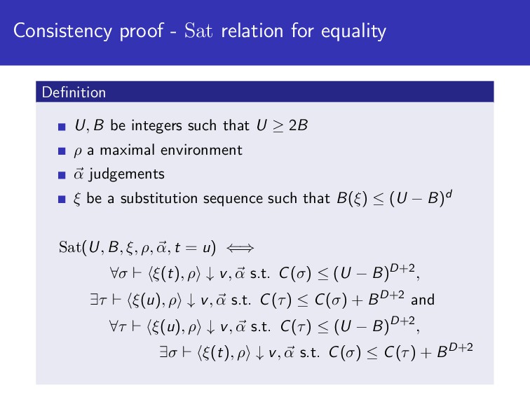
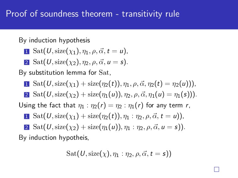
42. Proof of soundness theorem - transitivity rule By induction hypothesis 1 Sat(U, size(χ1), η1, ρ, α, t = u), 2 Sat(U, size(χ2), η2, ρ, α, u = s). By substitution lemma for Sat, 1 Sat(U, size(χ1) + size(η2(t)), η1, ρ, α, η2(t) = η2(u))), 2 Sat(U, size(χ2) + size(η1(u)), η2, ρ, α, η1(u) = η1(s))). Using the fact that η1 : η2(r) = η2 : η1(r) for any term r, 1 Sat(U, size(χ1) + size(η2(t)), η1 : η2, ρ, α, t = u)), 2 Sat(U, size(χ2) + size(η1(u)), η1 : η2, ρ, α, u = s)). By induction hypotheis, Sat(U, size(χ), η1 : η2, ρ, α, t = s))
43. Proof of soundness theorem - universal quantification Γ =⇒ t(x) = u(x) {x}(x), Γ =⇒ t(x) = u(x) For q, B([q/x] : ξ) ≤ (U − size(χ))d+1 s.t. FV(q) ⊆ {x}. By induction hypothesis, ∀ρ, Env(UD+2, ρ) → Sat(U, B, ξ, ρ, α, t(x) = u(x)) By substitution Sat(U, size(χ1) + size(t(ε) = u(ε)), ξ, ρ, α, t(q) = u(q)) Therefore, Sat(U, size(χ), [q/x] : ξ, ρ, α, t(x) = u(x))
44. PV1 - axioms A PV1-proof is a tree of sequents built by following axioms and rules. The subsystem PV1(D) is a system in which for all sequents Γ =⇒ ∆, the number of quantifiers plus the number of equations is bounded by D. t = u =⇒ t = u =⇒ t = t t = u =⇒ u = t t = u, u = s =⇒ t = s t1 = u1, . . . , tm = um =⇒ f (t1, . . . , tm) = f (u1, . . . , um) if f (x1, . . . , xm) = t is a defining axiom, =⇒ f (u1, . . . , um) = t(u1, . . . , um)
45. PV1 - structural and propositional rules Γ =⇒ ∆ φ, Γ =⇒ ∆ Γ =⇒ ∆ Γ =⇒ ∆, φ φ, φ, Γ =⇒ ∆ φ, Γ =⇒ ∆ Γ =⇒ ∆, φ, φ Γ =⇒ ∆, φ φi , Γ =⇒ ∆ φ1 ∧ φ2, Γ =⇒ ∆ (i = 1, 2) Γ =⇒ ∆, φ1 Σ =⇒ Π, φ2 Γ, Σ =⇒ ∆, Π, φ1 ∧ φ2 Γ =⇒ ∆, φ ¬φ, Γ =⇒ ∆ φ, Γ =⇒ ∆ Γ =⇒ ∆, ¬φ
46. PV1 - predicate and cut rules φ(t), Γ =⇒ ∆ ∀x.φ(x), Γ =⇒ ∆ Γ =⇒ ∆, φ(x) Γ =⇒ ∆, ∀x.φ(x) if x ∈ FV(Γ, ∆) φ(x), Γ =⇒ ∆ ∃x.φ(x), Γ =⇒ ∆ if x ∈ FV(Γ, ∆) Γ =⇒ ∆, φ(t) Γ =⇒ ∆, ∃x.φ(x) Γ =⇒ ∆, φ φ, Σ =⇒ Π Γ, Σ =⇒ ∆, Π
47. Embedding of PV− 1 (D) into PV− q (D) Definition Let φ1 ≡ Q1 =⇒ t1 = and φ2 ≡ Q2 =⇒ t2 = . Define φ⊥ ≡ Q⊥ =⇒ !t = u φ1 ∧ φ2 ≡ Q1, Q2 =⇒ t1&t2 = [⊥]q ≡ ⊥ = [t = u]q ≡ {i}(FV(t), FV(u)) =⇒ bit(t, i) ↔ bit(u, i) = [¬φ]q ≡ [φ]⊥ q [φ1 ∧ φ2]q ≡ [φ1]q ∧ [φ2]q [∀x.φ]q ≡ {x}(FV(φ)), [φ]q [∃x.φ]q ≡ x(FV(φ)), [φ]q.
48. Soundness of embedding of PV− 1 (D) into PV− q (D) Theorem (S2, Soundness of embedding) PV− 1 (D) φ1, . . . , φn =⇒ ψ1, . . . , ψm implies PV− q (D) [¬φ1 ∨ · · · ∨ ¬φn ∨ ψ1 ∨ · · · ∨ ψm]q
49. Soundness proof of embedding - contraction We need to prove [ψ ∨ φ]q from [ψ ∨ φ ∨ φ]q. Let [ψ]q ≡ Q1 =⇒ t = [φ]q ≡ Q2 =⇒ u = Q1, Q2, Q2 =⇒ t||u||u = Assume Q2 ≡ Q3, y(x). Q1, Q3, y(x), Q3 , y (x ) =⇒ t||u||u = . Let q(z) = p(z, y, y ). Q1, Q3, y(x), Q3 , y (x ) =⇒ t||u[q(u)/y] = Q1, Q3, Q3 , y(x), y (x ), z(x, y, y ) =⇒ t||u(z) = Q1, Q3, Q3 , z(x, x ), y(x), y (x) =⇒ t||u(z) = Q1, Q3, Q3 , z(x, x ) =⇒ t||u(z) = For the case Q2 ≡ Q3, {z}(x), the proof is easy.
50. Consistency of PV− 1 (D) + Ax Theorem Let A1 be the universal closure of conjunction of Ax. If A1 can be written in the language of PV− 1 (D), S2 proves the consistency of PV− 1 (D) + A1. To prove the theorem, we use the following lemma. Lemma (S1 2 ) Let t(x1, . . . , xn) be a term of type and ρ be an exact maximal environment. Assume that t(ρ(x1), . . . , ρ(xn)) = d in the standard interpretation. Then, there is a computation σ such that σ t, ρ ↓ d and nodes(σ) ≤ Pt(B(ρ)) for a polynomial Pt. Let P be a polynomial such that P(|n1| + · · · + |nm|) ≤ |t(n1, . . . , nm)| for any term t which appears in Ax.
51. Proof of consistency of PV− 1 (D) + Ax Argue inside S2. A is embedded into PV− q (D) as tA1 = . If PV− 1 (D) + Ax is inconsistent, we have PV− q (D) i1, . . . , ik =⇒ tA1 (i1, . . . , ik) = ⊥ Soundness of PV− q (D) and by definition of Sat, Sat(2size(π), size(π), [ ], tA1 (u1, . . . , uk) = ⊥) Therefore, there is a computation σ of tA1 (u1, . . . , uk), [ ] ↓ ⊥. By Substititon Lemma I, there is a maximal environment ρ and a computation σ0 of tA1 (x), ρ ↓ ⊥. Let ρ ρ be an exact environment. Then, there is a computation σ1 of tA1 (x), ρ ↓ ⊥. By previous lemma, we can build a computation τ of tA1 (x), ρ ↓ with enough large C(τ), which is against Compatibility Lemma.
52. Buss, S. R. and Ignjatovi´ c, A. (1995). Unprovability of consistency statements in fragments of bounded arithmetic. Annals of pure and applied Logic, 74:221–244. Krynicki, M. and Mostowski, M. (1995). Henkin quantifiers. In Quantifiers: logics, models and computation, pages 193–262. Springer. Takeuti, G. (1996). Incompleteness theorems and Si 2 versus Si+1 2 . In Logic Colloquium ’96: Proceedings of the Colloquium held in San Sebasti´ an, Spain, July 9-15, 1996, volume 12 of Lecture notes in logic, pages 247–261.