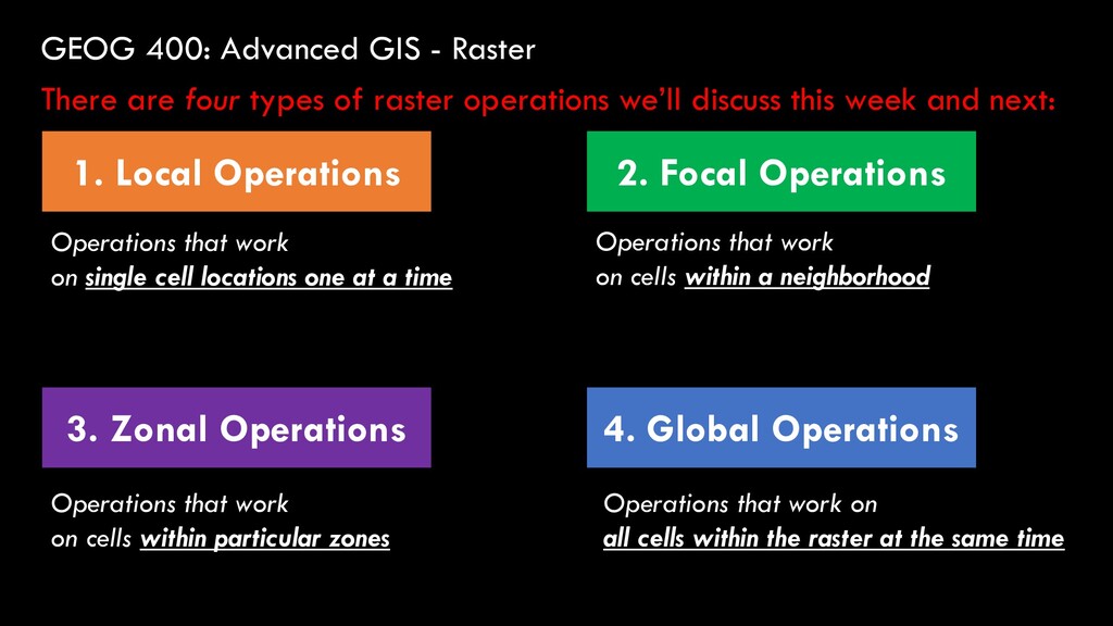
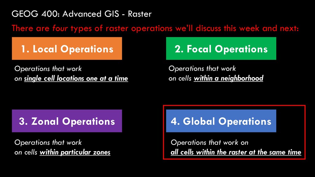
Global Operations 2. Focal Operations 3. Zonal Operations There are four types of raster operations we’ll discuss this week and next: Operations that work on single cell locations one at a time Operations that work on cells within a neighborhood Operations that work on cells within particular zones Operations that work on all cells within the raster at the same time
Global Operations 2. Focal Operations 3. Zonal Operations There are four types of raster operations we’ll discuss this week and next: Operations that work on single cell locations one at a time Operations that work on cells within a neighborhood Operations that work on cells within particular zones Operations that work on all cells within the raster at the same time
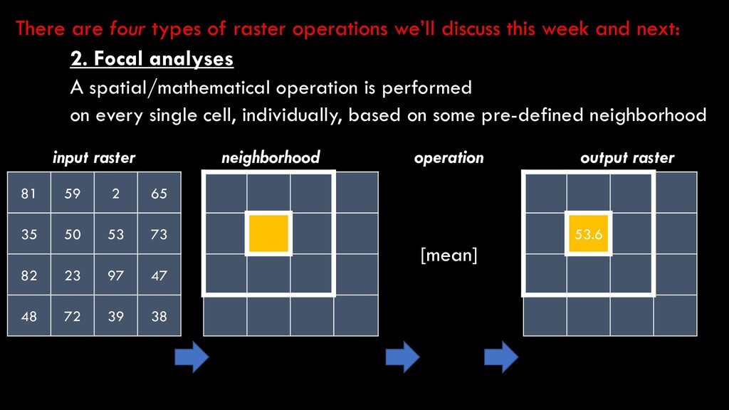
97 47 48 72 39 38 input raster operation [mean] output raster 53.6 neighborhood 2. Focal analyses A spatial/mathematical operation is performed on every single cell, individually, based on some pre-defined neighborhood There are four types of raster operations we’ll discuss this week and next:
3. Zonal analyses A spatial/mathematical operation is performed on groups of cells at the same time, based on some pre-defined neighborhood There are four types of raster operations we’ll discuss this week and next: input raster operation output raster neighborhood 81 59 2 65 35 50 53 73 82 23 97 47 48 72 39 38
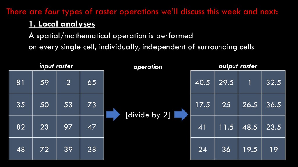
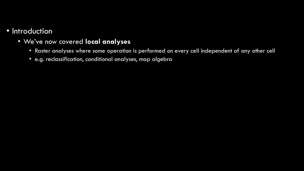
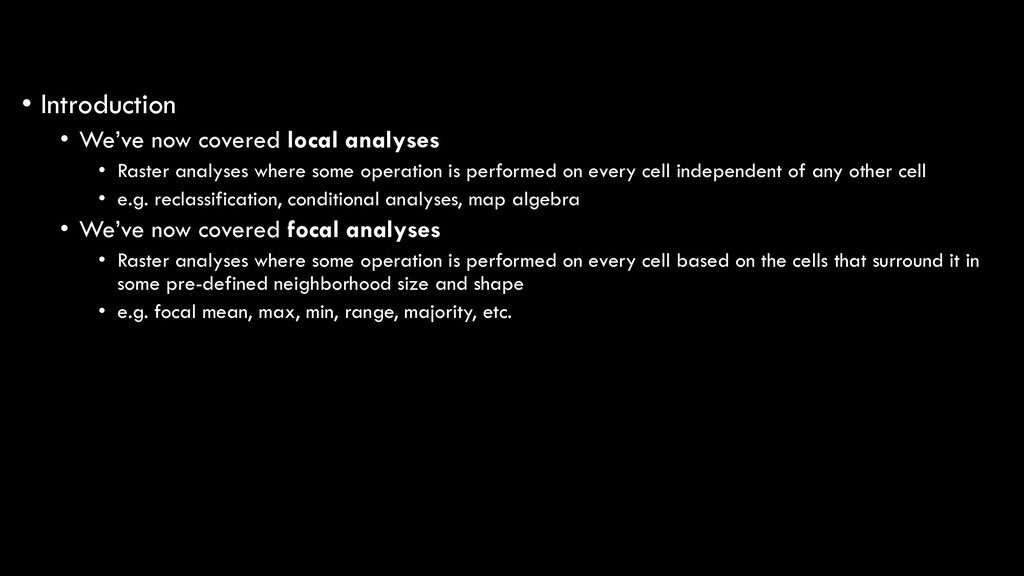
analyses where some operation is performed on every cell independent of any other cell • e.g. reclassification, conditional analyses, map algebra • We’ve now covered focal analyses • Raster analyses where some operation is performed on every cell based on the cells that surround it in some pre-defined neighborhood size and shape • e.g. focal mean, max, min, range, majority, etc.
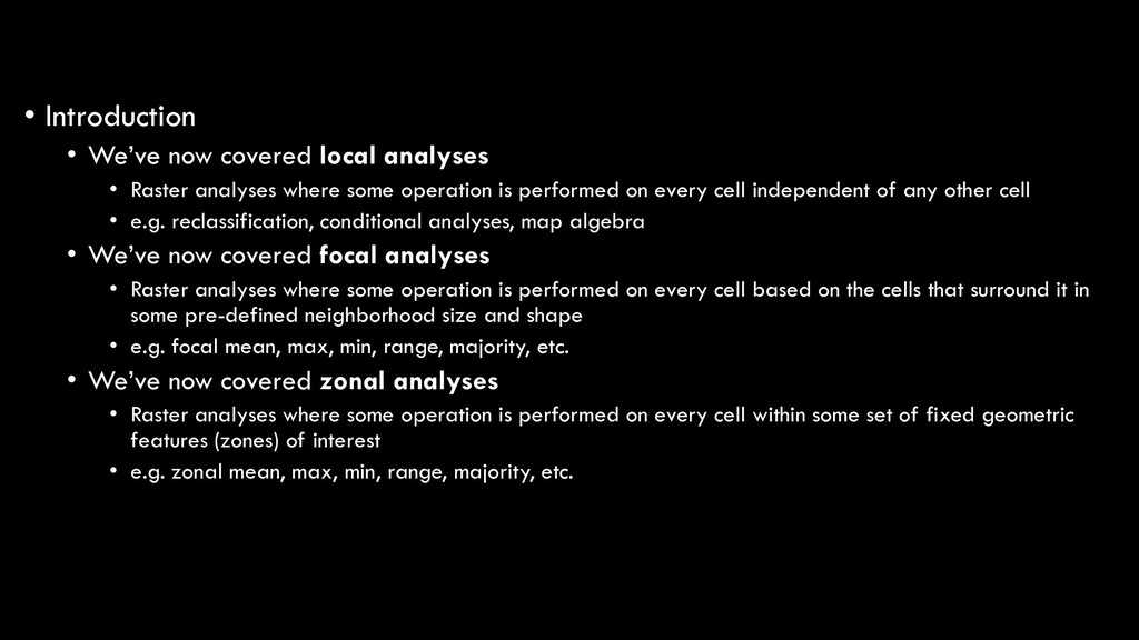
analyses where some operation is performed on every cell independent of any other cell • e.g. reclassification, conditional analyses, map algebra • We’ve now covered focal analyses • Raster analyses where some operation is performed on every cell based on the cells that surround it in some pre-defined neighborhood size and shape • e.g. focal mean, max, min, range, majority, etc. • We’ve now covered zonal analyses • Raster analyses where some operation is performed on every cell within some set of fixed geometric features (zones) of interest • e.g. zonal mean, max, min, range, majority, etc.
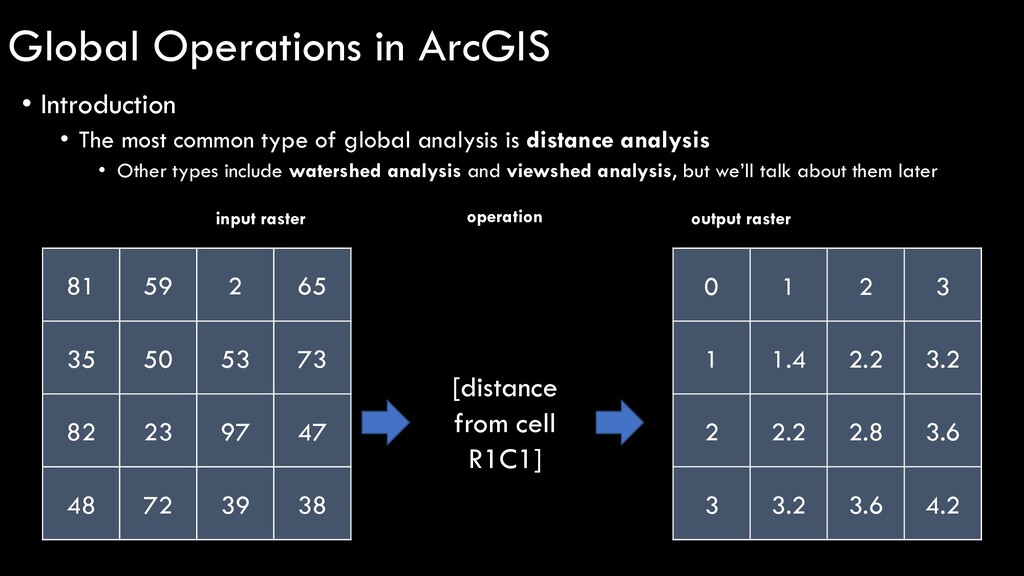
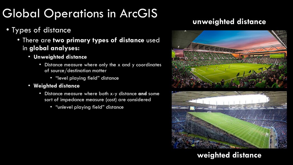
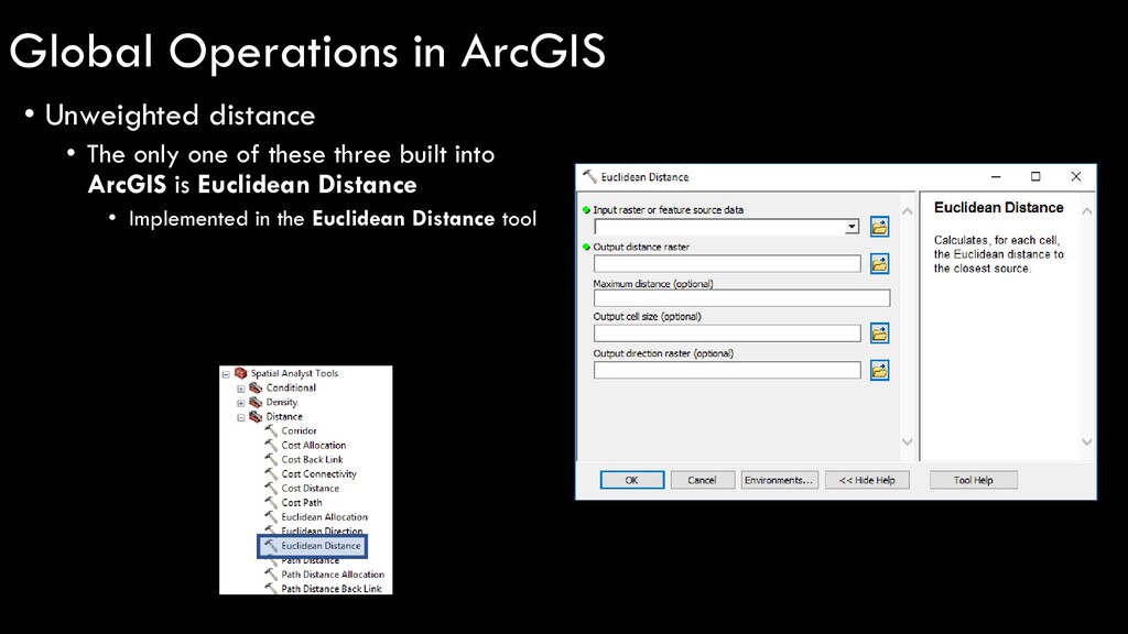
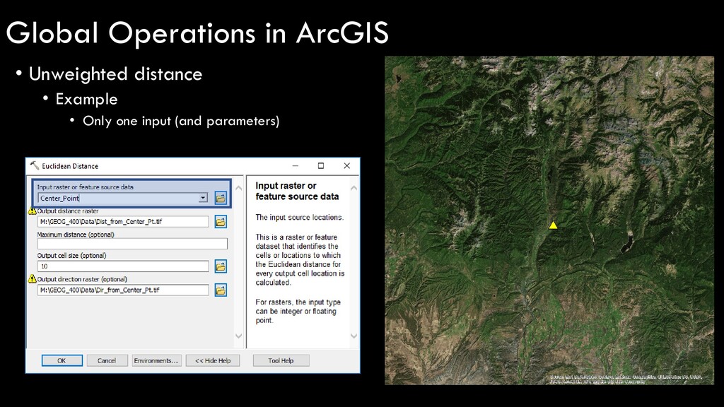
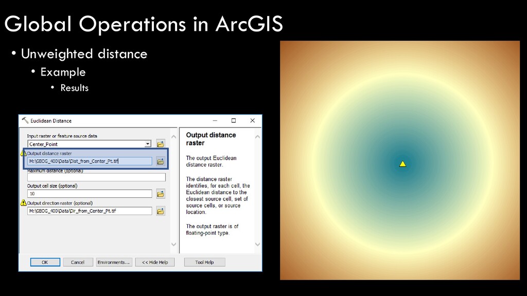
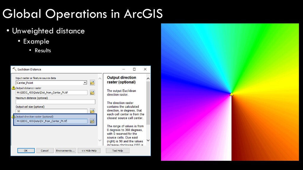
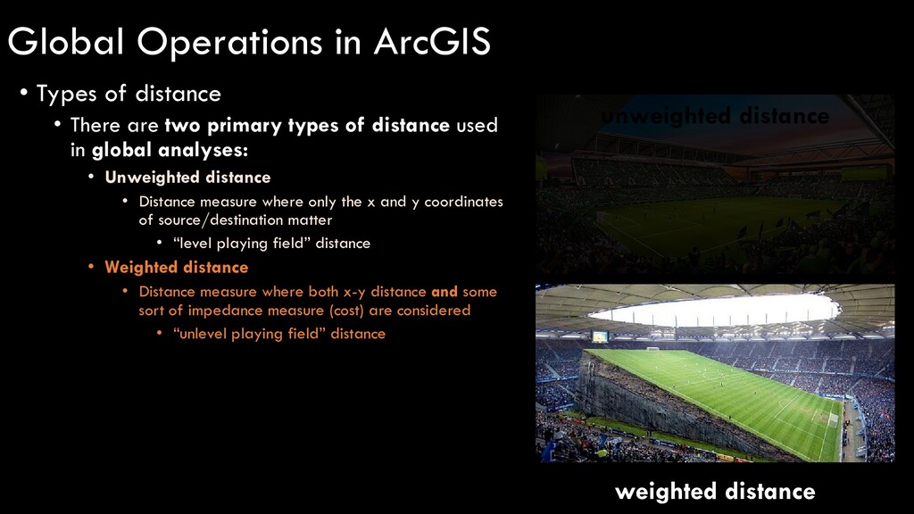
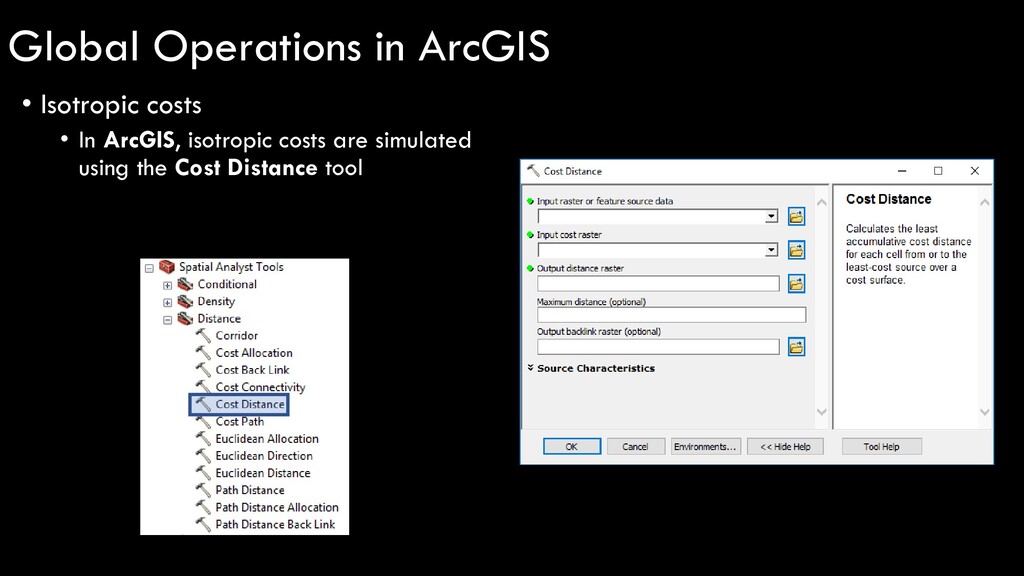
of distance used in global analyses: • Unweighted distance • Distance measure where only the x and y coordinates of source/destination matter • “level playing field” distance • Weighted distance • Distance measure where both x-y distance and some sort of impedance measure (cost) are considered • “unlevel playing field” distance unweighted distance weighted distance Global Operations in ArcGIS
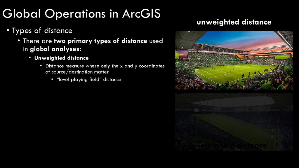
of distance used in global analyses: • Unweighted distance • Distance measure where only the x and y coordinates of source/destination matter • “level playing field” distance weighted distance Global Operations in ArcGIS unweighted distance
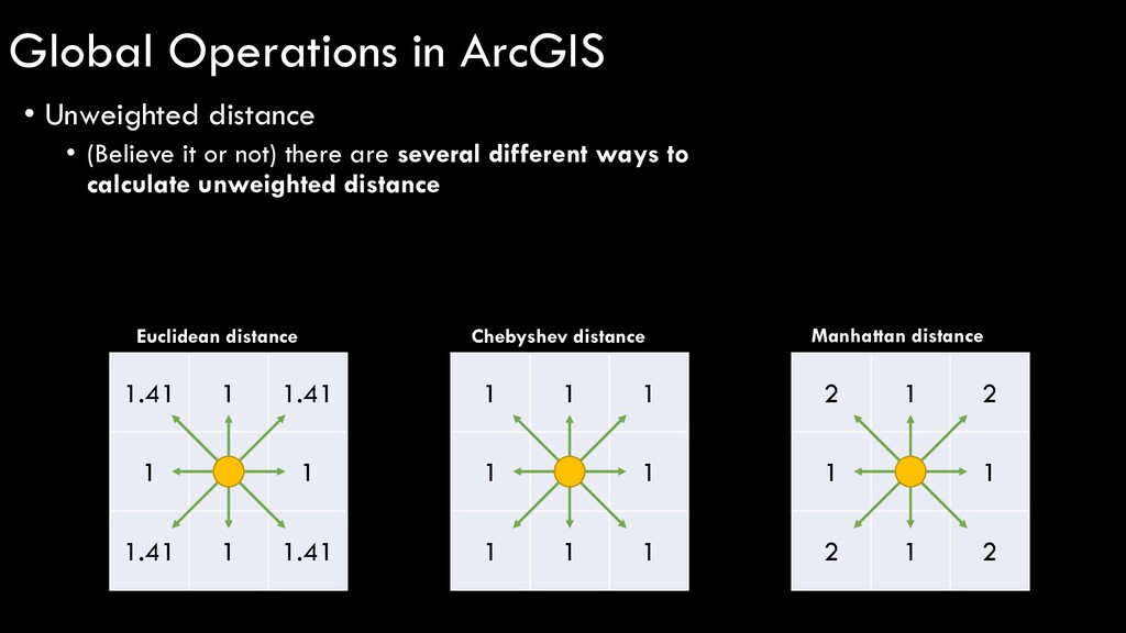
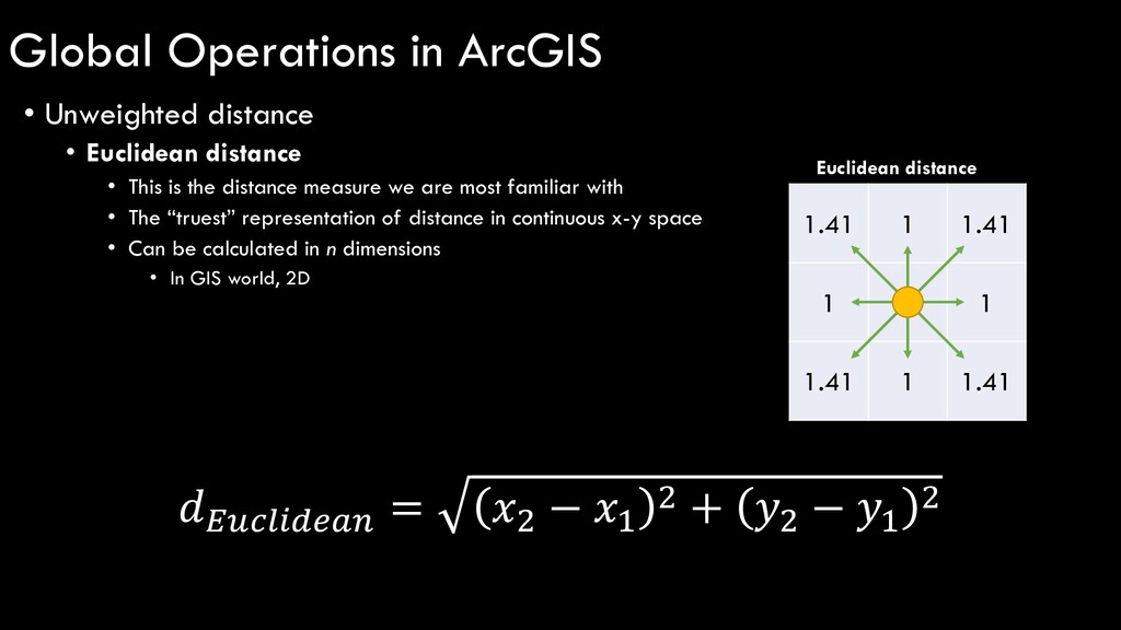
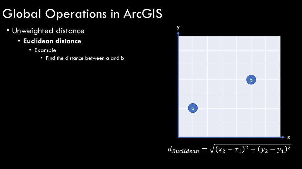
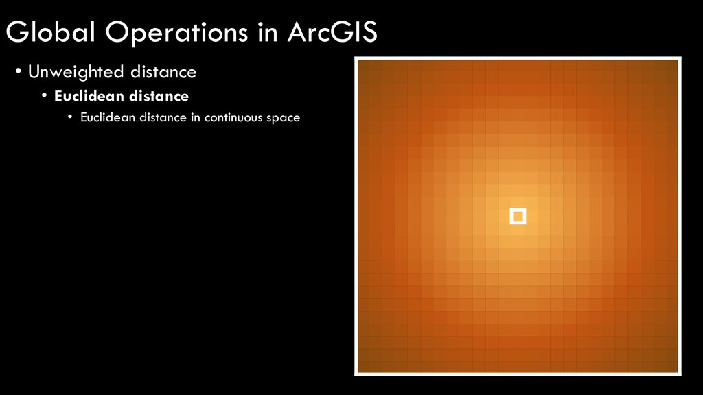
distance measure we are most familiar with • The “truest” representation of distance in continuous x-y space • Can be calculated in n dimensions • In GIS world, 2D 1.41 1 1.41 1 1 1.41 1 1.41 Euclidean distance = 2 − 1 2 + 2 − 1 2 Global Operations in ArcGIS
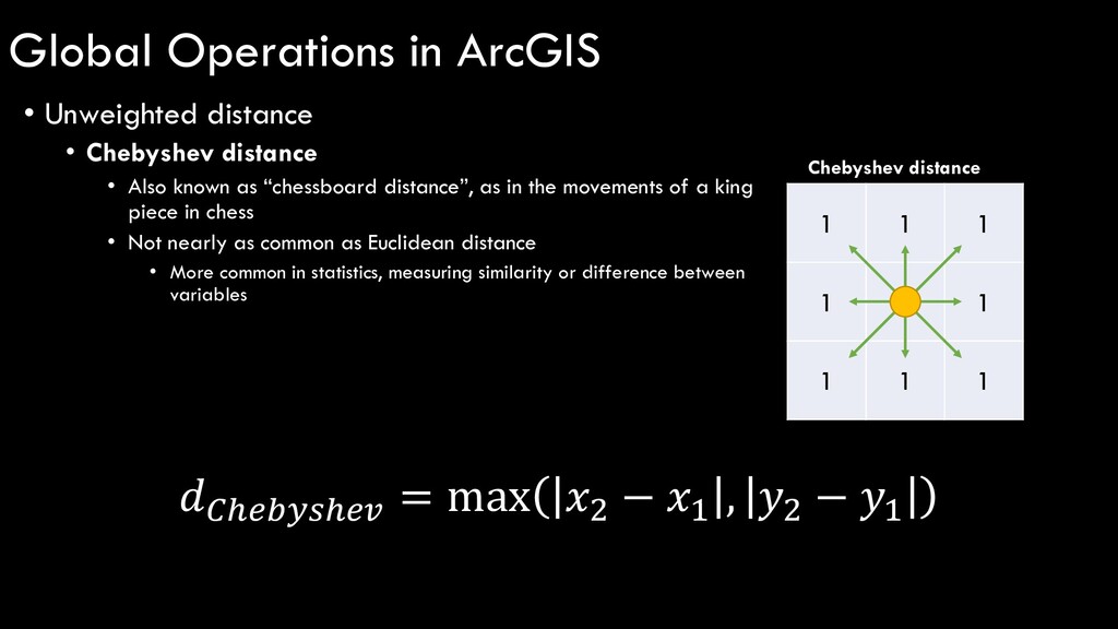
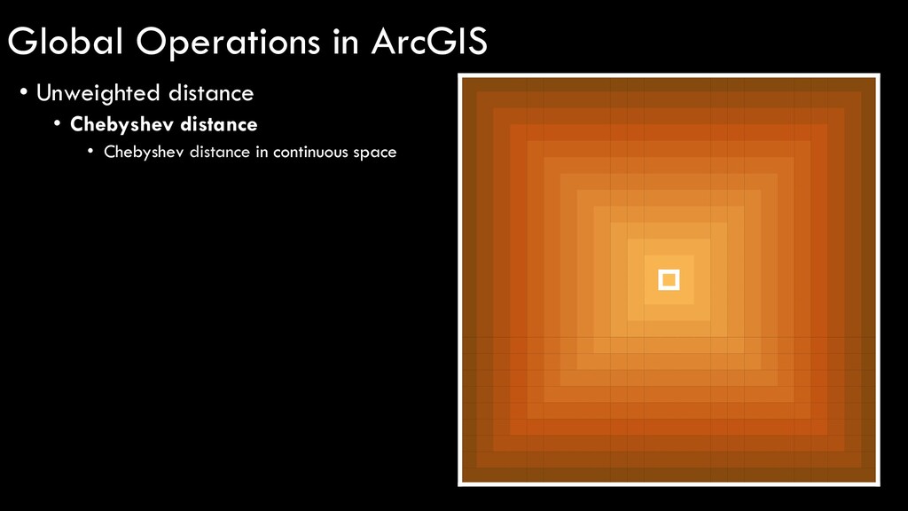
“chessboard distance”, as in the movements of a king piece in chess • Not nearly as common as Euclidean distance • More common in statistics, measuring similarity or difference between variables 𝐶𝐶𝐶𝐶 = max 2 − 1 , 2 − 1 1 1 1 1 1 1 1 1 Chebyshev distance Global Operations in ArcGIS
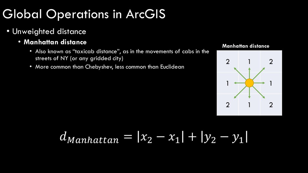
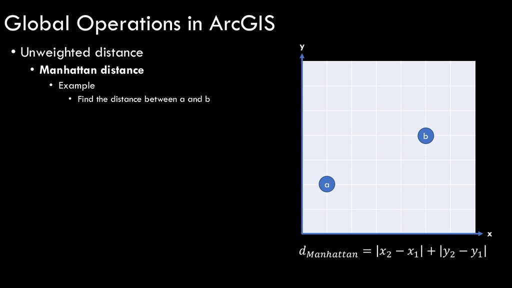
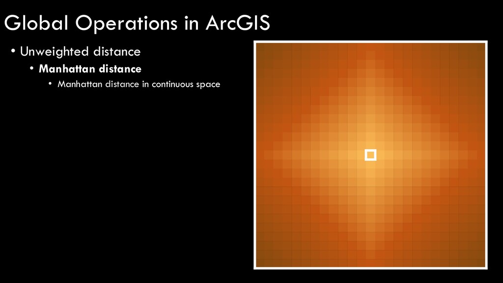
“taxicab distance”, as in the movements of cabs in the streets of NY (or any gridded city) • More common than Chebyshev, less common than Euclidean 𝑀𝑀𝑀𝑀𝑀𝑀𝑀𝑀𝑀𝑀𝑀 = 2 − 1 + 2 − 1 2 1 2 1 1 2 1 2 Manhattan distance Global Operations in ArcGIS
of distance used in global analyses: • Unweighted distance • Distance measure where only the x and y coordinates of source/destination matter • “level playing field” distance • Weighted distance • Distance measure where both x-y distance and some sort of impedance measure (cost) are considered • “unlevel playing field” distance unweighted distance weighted distance Global Operations in ArcGIS
of distance used in global analyses: • Unweighted distance • Distance measure where only the x and y coordinates of source/destination matter • “level playing field” distance • Weighted distance • Distance measure where both x-y distance and some sort of impedance measure (cost) are considered • “unlevel playing field” distance unweighted distance weighted distance Global Operations in ArcGIS
any number of ways in GIS… • Increased distance • e.g. traveling up a steep slope will effectively increase the distance traveled (c = sqrt(a2 + b2) • Increased “cost” • “cost” used to describe a variety of factors in GIS • Effort – e.g. physical toll it takes to travel over rough terrain • Difficulty – e.g. logistical challenge associated with navigating through an environment • Time – e.g. time it will take to build a trail through dense vegetation • Actual Cost – e.g. cost it will take to build a pipeline through varying property values • Other words for cost include impedance and friction Global Operations in ArcGIS
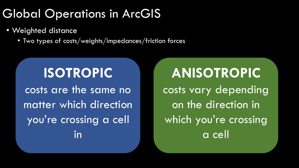
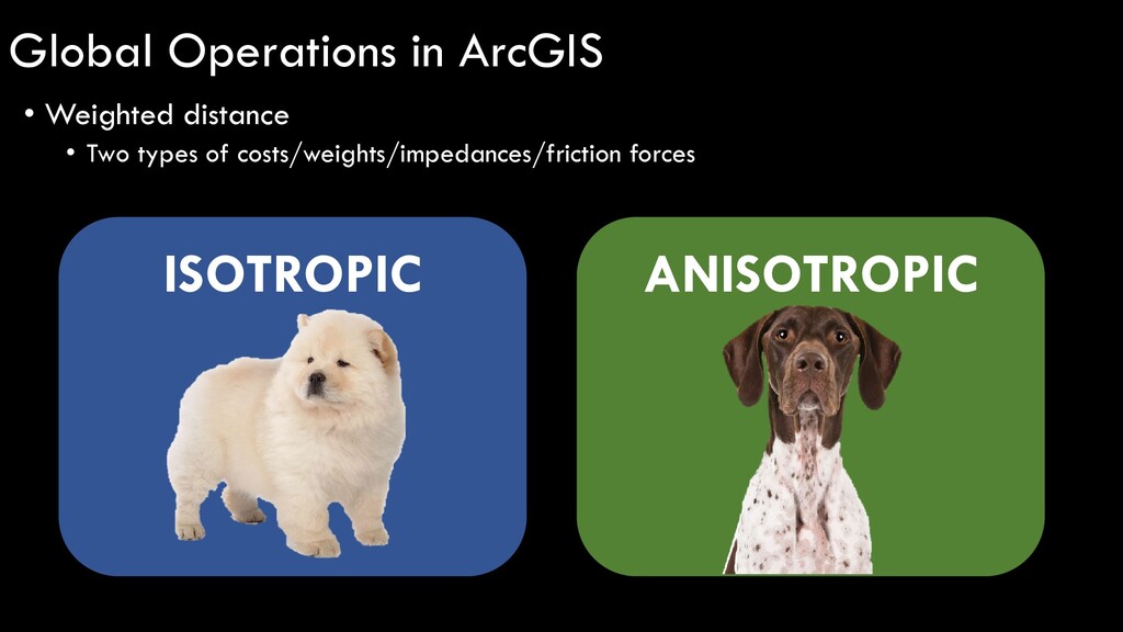
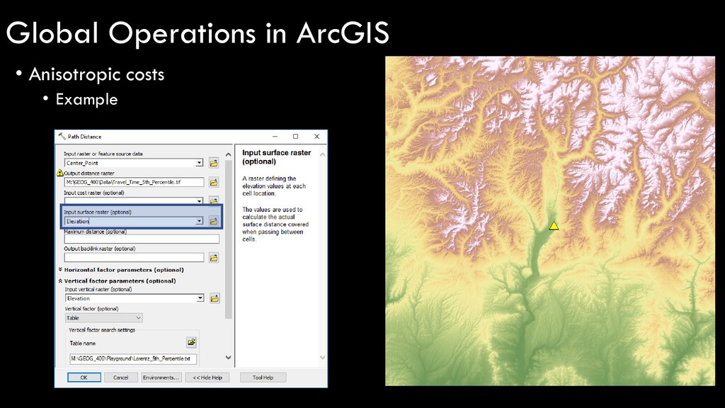
costs are the same no matter which direction you’re crossing a cell in ANISOTROPIC costs vary depending on the direction in which you’re crossing a cell Global Operations in ArcGIS
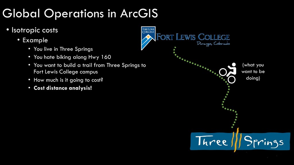
Springs • You hate biking along Hwy 160 • You want to build a trail from Three Springs to Fort Lewis College campus • How much is it going to cost? • Cost distance analysis! (what you want to be doing) Global Operations in ArcGIS
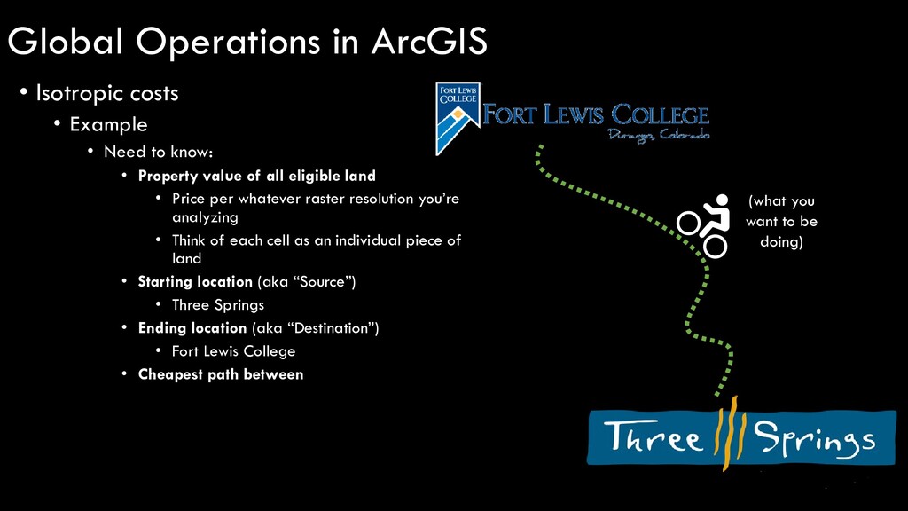
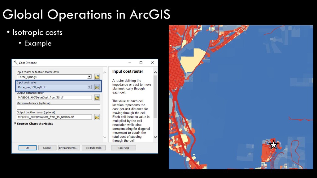
Property value of all eligible land • Price per whatever raster resolution you’re analyzing • Think of each cell as an individual piece of land • Starting location (aka “Source”) • Three Springs • Ending location (aka “Destination”) • Fort Lewis College • Cheapest path between (what you want to be doing) Global Operations in ArcGIS
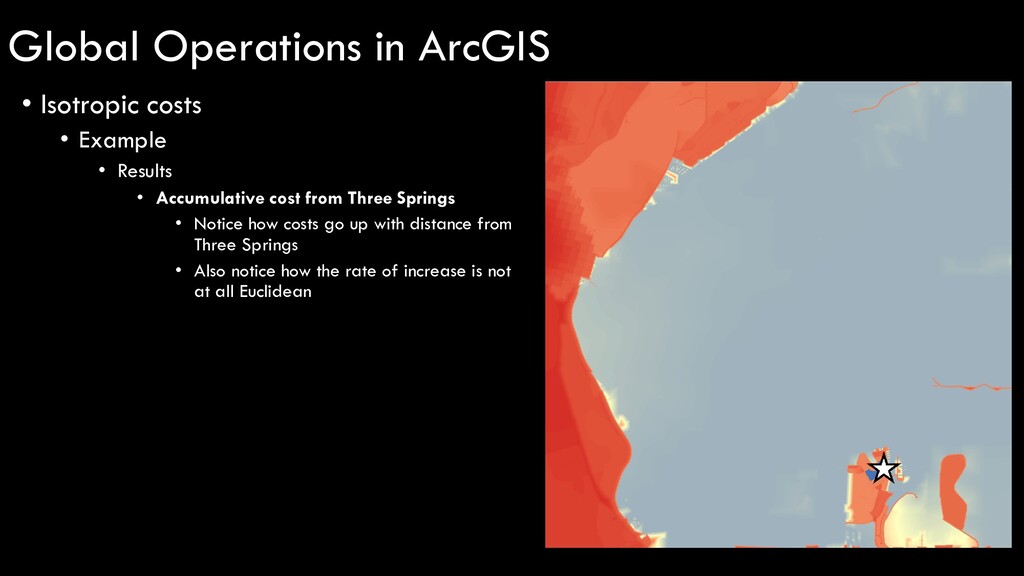
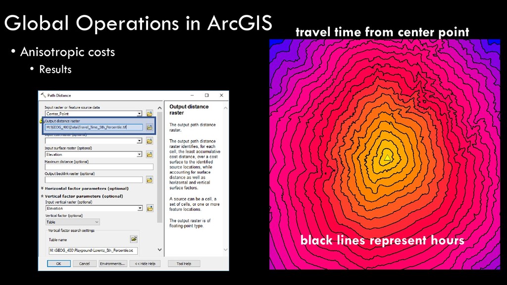
from Three Springs • Notice how costs go up with distance from Three Springs • Also notice how the rate of increase is not at all Euclidean Global Operations in ArcGIS
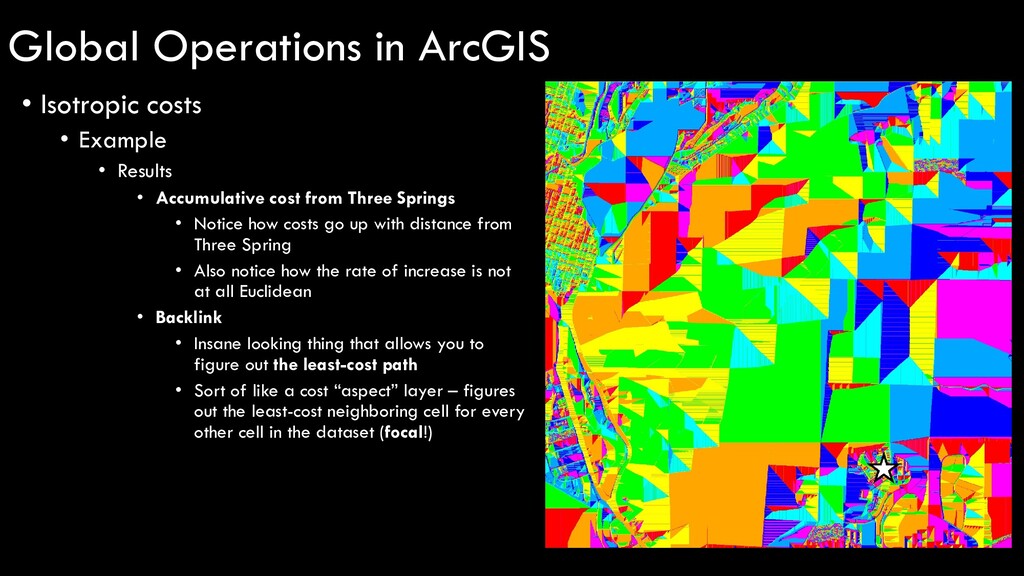
from Three Springs • Notice how costs go up with distance from Three Spring • Also notice how the rate of increase is not at all Euclidean • Backlink • Insane looking thing that allows you to figure out the least-cost path • Sort of like a cost “aspect” layer – figures out the least-cost neighboring cell for every other cell in the dataset (focal!) Global Operations in ArcGIS
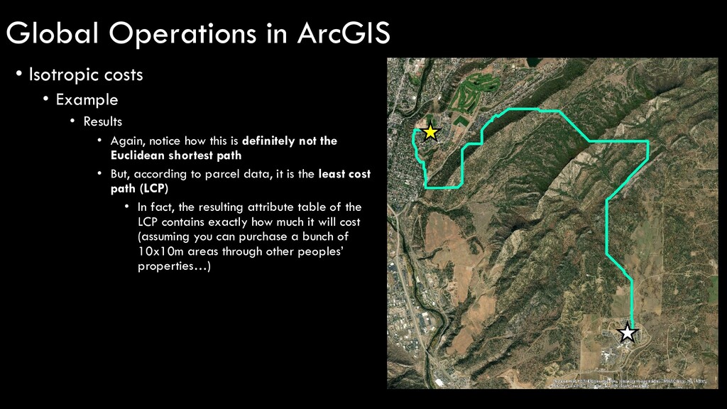
how this is definitely not the Euclidean shortest path • But, according to parcel data, it is the least cost path (LCP) • In fact, the resulting attribute table of the LCP contains exactly how much it will cost (assuming you can purchase a bunch of 10x10m areas through other peoples’ properties…) Global Operations in ArcGIS
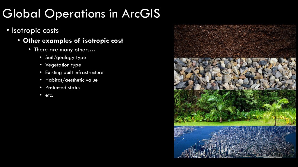
There are many others… • Soil/geology type • Vegetation type • Existing built infrastructure • Habitat/aesthetic value • Protected status • etc. Global Operations in ArcGIS
costs are the same no matter which direction you’re crossing a cell in ANISOTROPIC costs vary depending on the direction in which you’re crossing a cell Global Operations in ArcGIS
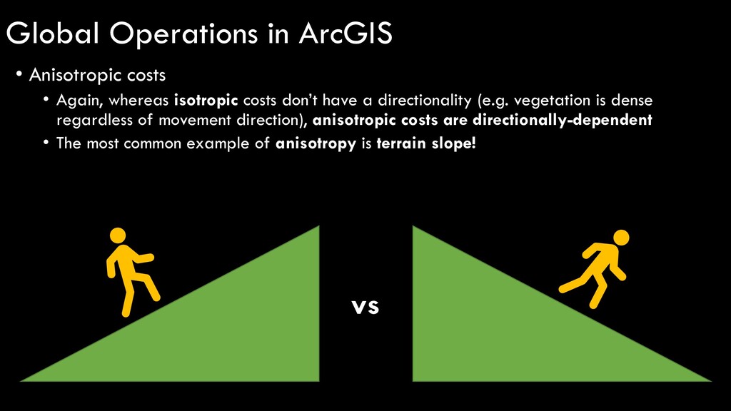
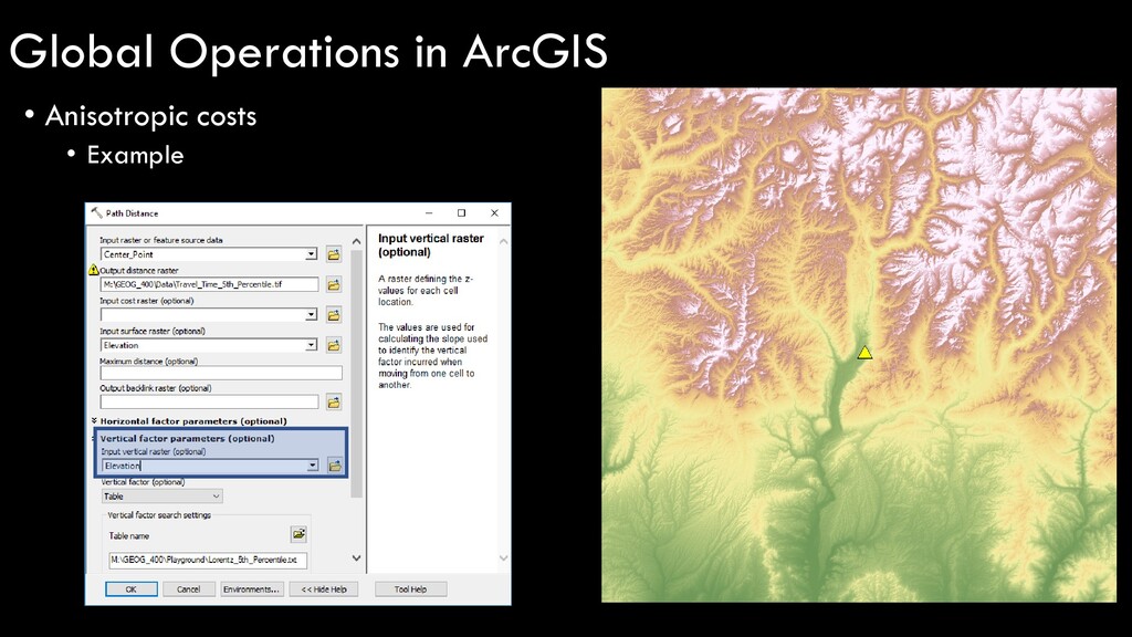
a directionality (e.g. vegetation is dense regardless of movement direction), anisotropic costs are directionally-dependent • The most common example of anisotropy is terrain slope! vs Global Operations in ArcGIS
themselves in two ways: • Increased travel distance • By traveling on sloped terrain, you are not simply moving in the x-y direction, you’re also moving up and downhill • a2 + b2 = c2 • Increased travel effort/time • Steeper slopes, generally more physically demanding • However, the effects of uphill travel on effort/time are not identical to those of downhill travel – anisotropy! Global Operations in ArcGIS
ground distance must include the effects of slope • Most distance estimators calculate distance based on x-y alone (e.g. Euclidean distance) • Navigation apps like Google Maps, AllTrails, etc. • Most analyses in ArcGIS Global Operations in ArcGIS
effects of slope are fairly negligible for most applications • Durango to Silverton example • Horizontal distance • 48.2 miles • Vertical distance • Silverton: 9318’ • Durango: 6512’ • Difference = 2806’ • Slope distance • sqrt(48.22+0.532) = 48.203 miles • 0.003 miles = 16 feet Durango Silverton 48.2 miles 0.53 miles Global Operations in ArcGIS
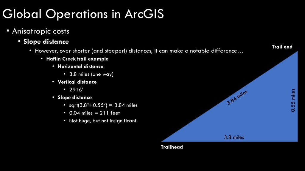
(and steeper!) distances, it can make a notable difference… • Haflin Creek trail example • Horizontal distance • 3.8 miles (one way) • Vertical distance • 2916’ • Slope distance • sqrt(3.82+0.552) = 3.84 miles • 0.04 miles = 211 feet • Not huge, but not insignificant! Trailhead Trail end 3.8 miles 0.55 miles Global Operations in ArcGIS
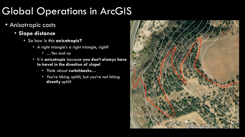
this anisotropic? • A right triangle’s a right triangle, right? • …Yes and no • It is anisotropic because you don’t always have to travel in the direction of slope! • Think about switchbacks… • You’re hiking uphill, but you’re not hiking directly uphill Global Operations in ArcGIS
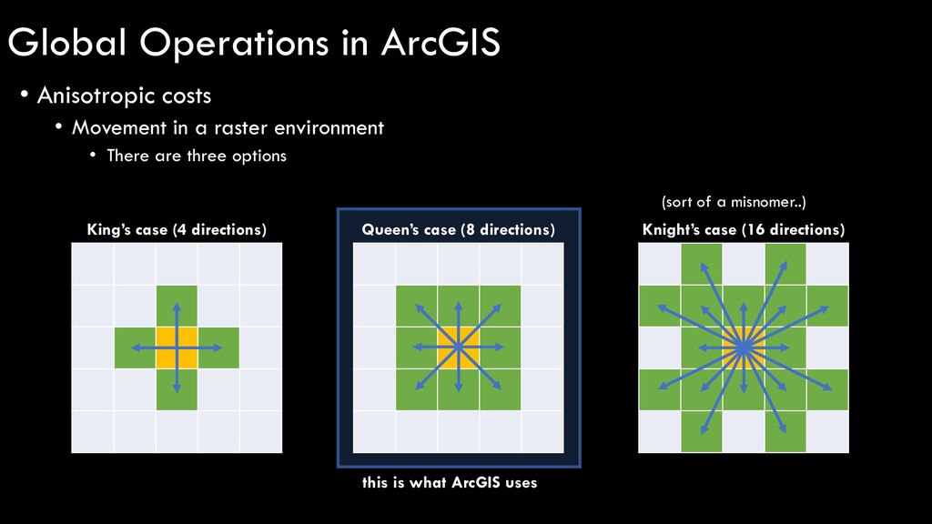
There are three options King’s case (4 directions) Queen’s case (8 directions) Knight’s case (16 directions) (sort of a misnomer..) this is what ArcGIS uses Global Operations in ArcGIS
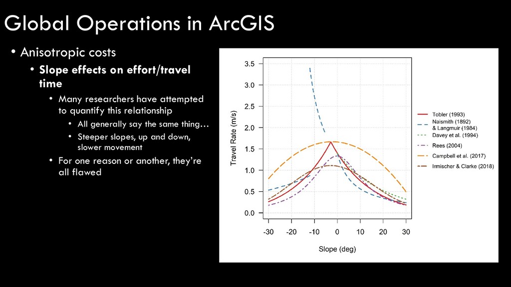
Many researchers have attempted to quantify this relationship • All generally say the same thing… • Steeper slopes, up and down, slower movement • For one reason or another, they’re all flawed Global Operations in ArcGIS
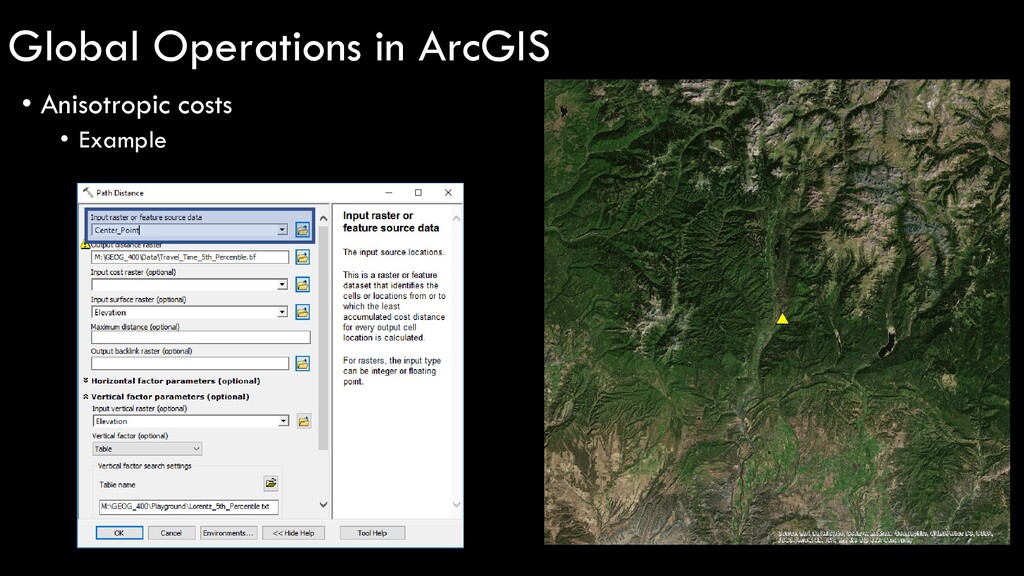
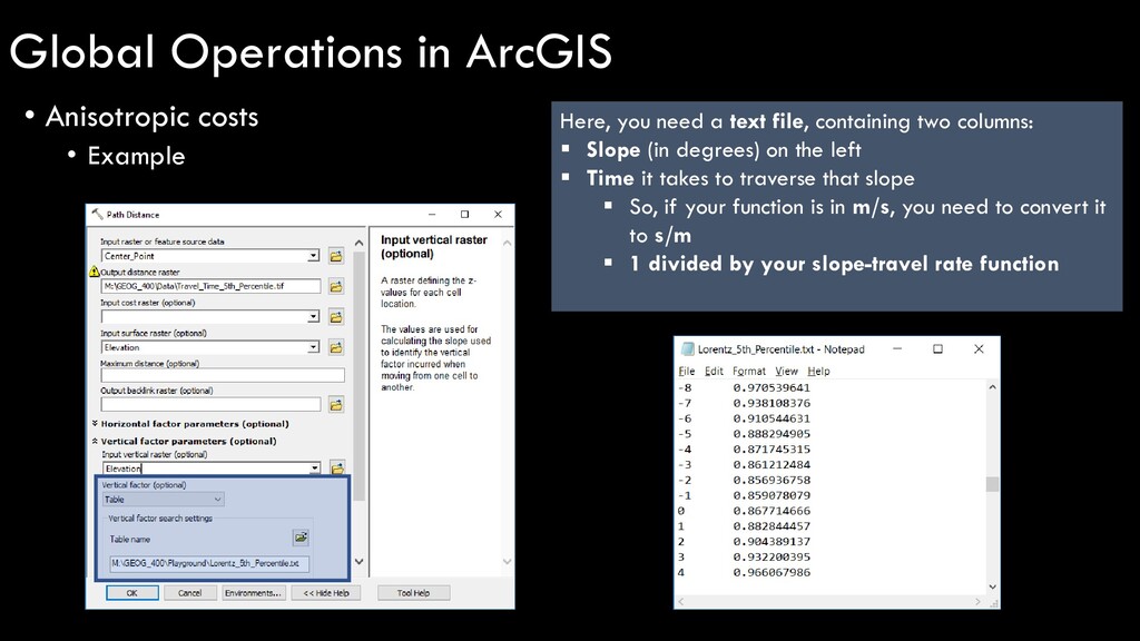
file, containing two columns: Slope (in degrees) on the left Time it takes to traverse that slope So, if your function is in m/s, you need to convert it to s/m 1 divided by your slope-travel rate function Global Operations in ArcGIS
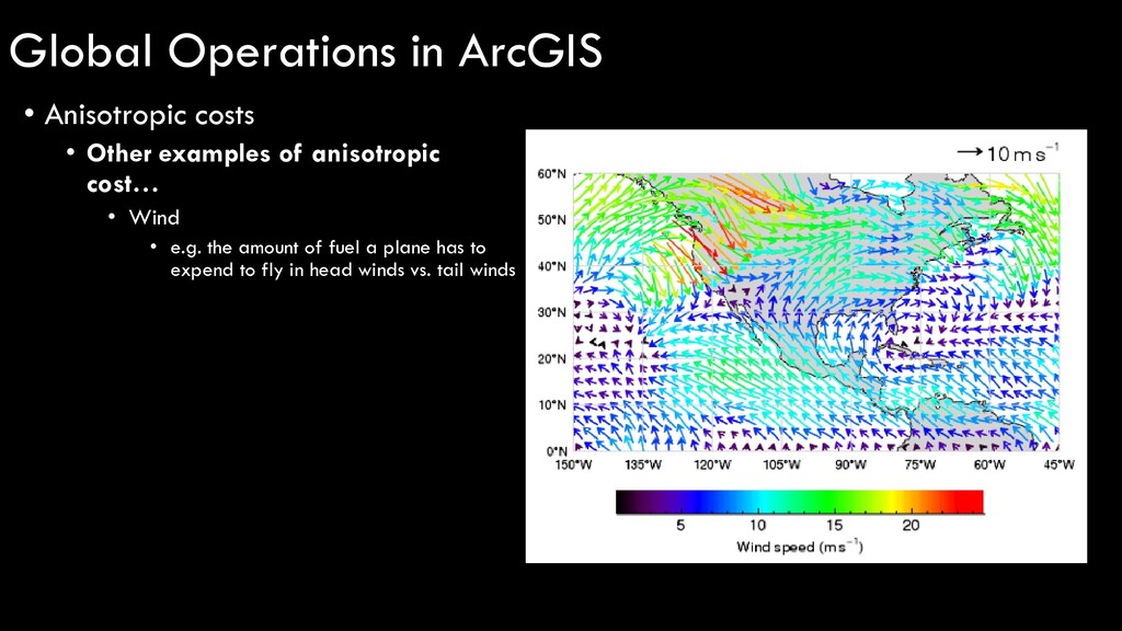
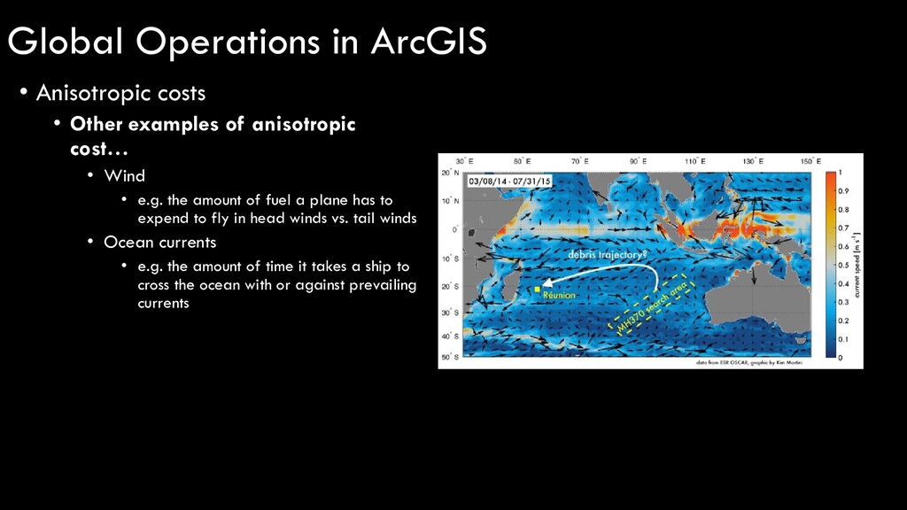
Wind • e.g. the amount of fuel a plane has to expend to fly in head winds vs. tail winds • Ocean currents • e.g. the amount of time it takes a ship to cross the ocean with or against prevailing currents Global Operations in ArcGIS
![[mean] 53.6 53.6 53.6 53.6 53.6 53.6 53.6 53.6 53.6](https://files.speakerdeck.com/presentations/a8a73c41e3ad494cba4bdffdff084d75/slide_5.jpg)