Lecture slides for POM 1-6

生産管理技術1の講義6のスライドです．

Transcript

1. © Hajime Mizuyama Production & Operations Management #1 @AGU Lec.6: Production Planning and Linear Programming • What is production planning? • How to formulate it mathematically? • Linear programming approach to production planning
2. © Hajime Mizuyama Course Schedule #1 Date Contents Outline of production management (1): How to conceptualize production systems Outline of production management (2): Framework of production planning and control Inventory control and management (1): Economic order quantity (EOQ) and the role of safety stock Inventory control and management (2): Conventional inventory control models Production planning and linear programming MRP (1): Bill of materials (BOM), priority planning, capacity planning, etc. MRP (2): Lot sizing and dynamic order quantity (DOQ)
3. © Hajime Mizuyama Production Planning When Where How much of what (workload) Planning horizon Time unit Resource Production capacity Planning cycle A decision making on • When • Where • How much of what products should be produced (or operations should be carried out). Rolling horizon A shorter cycle time than the planning horizon is used, to make it easier to incorporate realized uncertainties into the plan.
4. © Hajime Mizuyama Production Planning When Where How much of what (workload) Planning horizon Time unit Planning cycle X3 X1 X2 A decision making on • When • Where • How much of what products should be produced (or operations should be carried out). Rolling horizon A shorter cycle time than the planning horizon is used, to make it easier to incorporate realized uncertainties into the plan.
5. © Hajime Mizuyama Decision variables • Production quantities of products 1, 2, …, N Objective function • Maximize the profit (contribution). Constraints • Available machine-hours/man-hours • Available materials • Limited demand • Non-negative constraints, etc. Mathematical Formulation: Single-Period Problem #1
6. © Hajime Mizuyama Decision variables • 𝑋! , 𝑋" , ⋯ , 𝑋# Objective function • 𝑃 = ∑$%! # 𝑝$ ( 𝑋$ ⇒ Maximize Constraints • ∑$%! # ℎ$& ( 𝑋$ ≤ 𝐻& (𝑚 = 1, 2, ⋯ , 𝑀) • ∑$%! # 𝑏$' ( 𝑋$ ≤ 𝐵' (𝑘 = 1, 2, ⋯ , 𝐾) • 𝐿$ ≤ 𝑋$ ≤ 𝑈$ (𝑛 = 1, 2, ⋯ , 𝑁) • 𝑋$ ≥ 0 (𝑛 = 1, 2, ⋯ , 𝑁) Mathematical Formulation: Single-Period Problem #2
7. © Hajime Mizuyama Illustrative Example: Single-Period Problem #1 We should determine the quantities of products A and B to be produced in the next time period (month), so as to maximize the profit. The marginal profit per unit is $4 for product A and $3 for B. Thus, the objective function can be expressed as below: 𝑓 = 4𝑋! + 3𝑋" where 𝑋! and 𝑋" represent the numbers of products A and B to be produced, respectively.
8. © Hajime Mizuyama Illustrative Example: Single-Period Problem #2 Machine-hours constraint: The machine-hours per unit is 1 for product A and 4 for B, and the total machine-hours available next period is 5200. 𝑋! + 4𝑋" ≤ 5200 Man-hours constraint: The man-hours per unit is 14 for product A and 4 for B, and the total man-hours available next period is 15600. 14𝑋! + 4𝑋" ≤ 15600 Material constraint: A special material is required only for A (only 1000 units available). 𝑋! ≤ 1000 Non-negative constraints: The production volumes cannot be negative. 𝑋! , 𝑋" ≥ 0
9. © Hajime Mizuyama Decision variables • 𝑋! , 𝑋" Objective function • 𝑓 = 4𝑋! + 3𝑋" ⇒ Maximize Constraints • 𝑋! + 4𝑋" ≤ 5200 • 14𝑋! + 4𝑋" ≤ 15600 • 𝑋! ≤ 1000 • 𝑋! , 𝑋" ≥ 0 Illustrative Example: Mathematical Formulation Eq.(2) Eq.(4) Eq.(3) Eq.(5) Eq.(1) When all the objective function and constraints are linear functions of the decision variables, the problem is called a linear programming.
10. © Hajime Mizuyama 𝑋! + 4𝑋" ≤ 5200 14𝑋! + 4𝑋" ≤ 15600 𝑋! ≤ 1000 𝑋! , 𝑋" ≥ 0 Graphical Approach to Linear Programming #1 Eq.(2) Eq.(4) Eq.(3) Eq.(5) 0 𝑋! 𝑋"
11. © Hajime Mizuyama 𝑋! + 4𝑋" ≤ 5200 Eq.(2) 14𝑋! + 4𝑋" ≤ 15600 𝑋! ≤ 1000 Eq.(4) Eq.(3) 𝑋! , 𝑋" ≥ 0 Eq.(5) Eq.(4) is satisfied. Eq.(4) is not satisfied. Graphical Approach to Linear Programming #2 0 1000 𝑋! 𝑋" 𝑋! = 1000
12. © Hajime Mizuyama 𝑋! + 4𝑋" ≤ 5200 14𝑋! + 4𝑋" ≤ 15600 𝑋! ≤ 1000 𝑋! , 𝑋" ≥ 0 Graphical Approach to Linear Programming #3 Eq.(2) and (4) are satisfied. Eq.(2) Eq.(4) Eq.(3) Eq.(5) 0 1000 𝑋! 𝑋" 𝑋! = 1000 𝑋! + 4𝑋" ≤ 5200
13. © Hajime Mizuyama Graphical Approach to Linear Programming #4 𝑋! + 4𝑋" ≤ 5200 Eq.(2) 14𝑋! + 4𝑋" ≤ 15600 Eq.(3) 𝑋! ≤ 1000 Eq.(4) 𝑋! , 𝑋" ≥ 0 Eq.(5) 0 1000 1300 𝑋! 𝑋" 𝑋! = 1000 𝑋! + 4𝑋" ≤ 5200 14𝑋! + 4𝑋" ≤ 15600
14. © Hajime Mizuyama Graphical Approach to Linear Programming #5 Contour lines of equal profit The profit is given by A contour line connecting (0, 800) and (600, 0) corresponds to f = 2400. $2400 $4800 𝑓 = 4𝑋! + 3𝑋" Eq.(1) A contour line connecting (0, 1600) and (1200, 0) represents f = 4800. 0 1200 1600 600 800 𝑋! 𝑋"
15. © Hajime Mizuyama • The optimal solution is on the contour line farthest away from the origin that is inside or on the border of the feasible region. • The figure shows that the optimal solution is on the line passing (800, 1100) and the corresponding profit is (4 ( 800) + (3 ( 1100) = $6500 • Thus, the optimal production volumes are 𝑋! = 800 and 𝑋" = 1100. $2400 $4800 $6500 Graphical Approach to Linear Programming #6 (800, 1100) 0 𝑋! 𝑋"
16. © Hajime Mizuyama Anticipation stock It arises due to front-loaded production for covering an anticipated future capacity shortage. In order to successfully arrange anticipation stock, the following functions are necessary: – Demand forecasting – Multi-period production planning Anticipation Stock and Multi-Period Planning Time Volume Capacity Demand forecast
17. © Hajime Mizuyama Decision variables • How many products 1, 2, …, N to be produced in periods 1, 2, …, T • Those to be carried over from periods 1, 2, …, T -1 Objective function • Maximize the profit minus inventory costs. Constraints • Available machine-hours/man-hours/materials • Limited demand • Non-negative constraints, etc. Mathematical Formulation: Multi-Period Problem #1
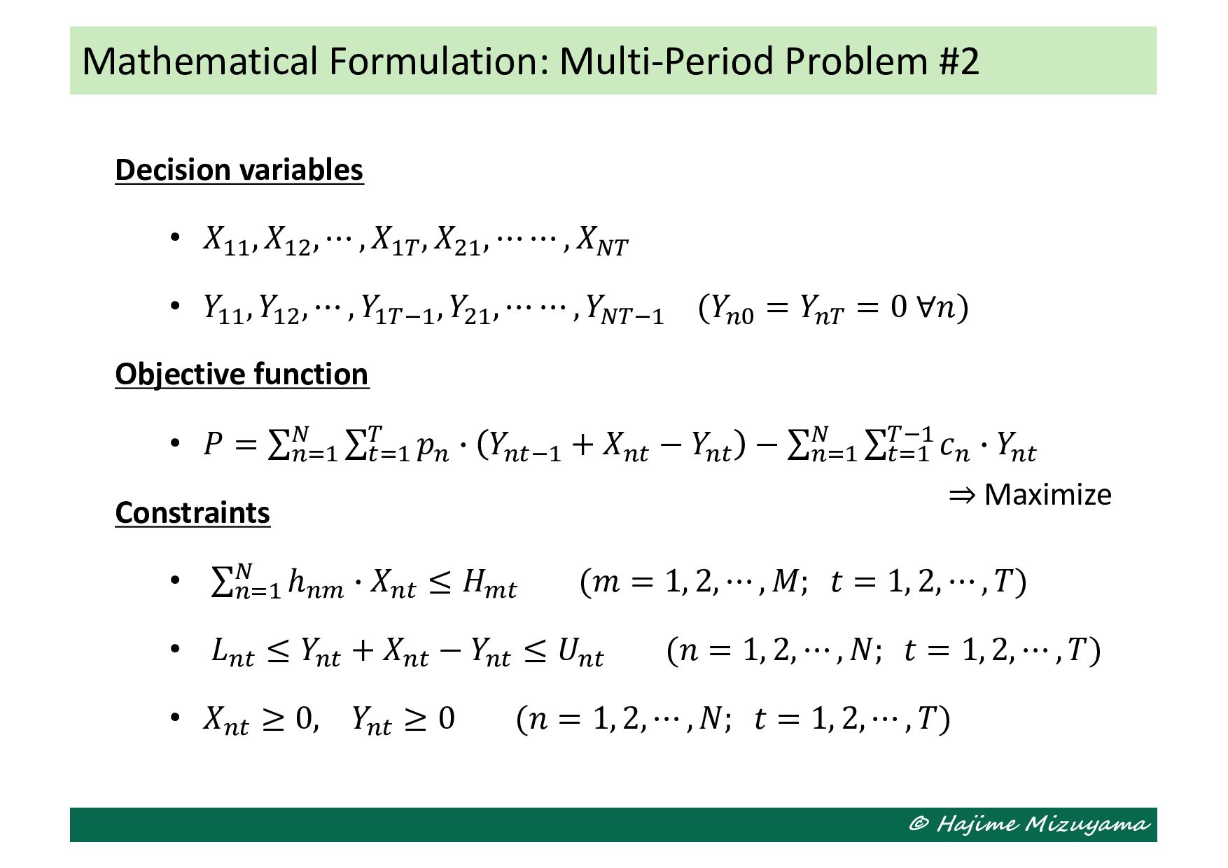
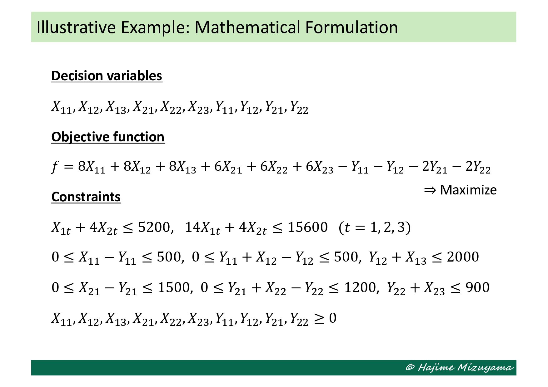
18. © Hajime Mizuyama Decision variables • 𝑋!! , 𝑋!" , ⋯ , 𝑋!( , 𝑋"! , ⋯ ⋯ , 𝑋#( • 𝑌!! , 𝑌!" , ⋯ , 𝑌!()! , 𝑌"! , ⋯ ⋯ , 𝑌#()! (𝑌$* = 𝑌$( = 0 ∀𝑛) Objective function • 𝑃 = ∑$%! # ∑+%! ( 𝑝$ ( 𝑌$+)! + 𝑋$+ − 𝑌$+ − ∑$%! # ∑+%! ()! 𝑐$ ( 𝑌$+ Constraints • ∑$%! # ℎ$& ( 𝑋$+ ≤ 𝐻&+ (𝑚 = 1, 2, ⋯ , 𝑀; 𝑡 = 1, 2, ⋯ , 𝑇) • 𝐿$+ ≤ 𝑌$+ + 𝑋$+ − 𝑌$+ ≤ 𝑈$+ (𝑛 = 1, 2, ⋯ , 𝑁; 𝑡 = 1, 2, ⋯ , 𝑇) • 𝑋$+ ≥ 0, 𝑌$+ ≥ 0 (𝑛 = 1, 2, ⋯ , 𝑁; 𝑡 = 1, 2, ⋯ , 𝑇) Mathematical Formulation: Multi-Period Problem #2 ⇒ Maximize
19. © Hajime Mizuyama Illustrative Example: Multi-Period Problem #1 We should determine the quantities of products A and B to be produced in the next three time periods (months). The marginal profit per unit and the inventory cost per unit per period are $8 and $1 for product A and $6 and $2 for B. Thus, the objective function can be expressed as below: 𝑓 = 8𝑋!! + 8𝑋!" + 8𝑋!, + 6𝑋"! + 6𝑋"" + 6𝑋", −𝑌!! − 𝑌!" − 2𝑌"! − 2𝑌"" where 𝑋!+ and 𝑌!+ represent the numbers of product A to be produced in and carried over from period t, and 𝑋"+ and 𝑌"+ those of product B.
20. © Hajime Mizuyama Illustrative Example: Multi-Period Problem #2 Resource constraint: Man-hours and machine-hours required per unit are 1 and 14 for A, and 4 and 4 for B, and there are only 5200 and 15600 available in total in each period. Demand constraint: Demand for products A and B are given as below. Non-negative constraints: The decision variables cannot be negative. t 1 2 3 A 500 500 2000 B 1500 1200 900
21. © Hajime Mizuyama Decision variables 𝑋!! , 𝑋!" , 𝑋!, , 𝑋"! , 𝑋"" , 𝑋", , 𝑌!! , 𝑌!" , 𝑌"! , 𝑌"" Objective function 𝑓 = 8𝑋!! + 8𝑋!" + 8𝑋!# + 6𝑋"! + 6𝑋"" + 6𝑋"# − 𝑌!! − 𝑌!" − 2𝑌"! − 2𝑌"" Constraints 𝑋!+ + 4𝑋"+ ≤ 5200, 14𝑋!+ + 4𝑋"+ ≤ 15600 (𝑡 = 1, 2, 3) 0 ≤ 𝑋!! − 𝑌!! ≤ 500, 0 ≤ 𝑌!! + 𝑋!" − 𝑌!" ≤ 500, 𝑌!" + 𝑋!, ≤ 2000 0 ≤ 𝑋"! − 𝑌"! ≤ 1500, 0 ≤ 𝑌"! + 𝑋"" − 𝑌"" ≤ 1200, 𝑌"" + 𝑋", ≤ 900 𝑋!! , 𝑋!" , 𝑋!, , 𝑋"! , 𝑋"" , 𝑋", , 𝑌!! , 𝑌!" , 𝑌"! , 𝑌"" ≥ 0 Illustrative Example: Mathematical Formulation ⇒ Maximize
22. © Hajime Mizuyama How to Solve LP with Excel #1
23. © Hajime Mizuyama How to Solve LP with Excel #2
24. © Hajime Mizuyama How to Solve LP with Excel #3
25. © Hajime Mizuyama How to Solve LP with Excel #4
26. © Hajime Mizuyama Supplemental material on how to solve LP problems using PuLP (a Python library) and accompanying free solver CBC is available from the following link. Push “Open in Colab” button, then you can test it in Google Colaboratory environment. https://github.com/j54854/myColab/blob/main/pom1_6.ipynb How to Solve LP with PuLP (& CBC Solver)