University of Waterlo 200 University Avenue We Waterloo, ON, Canada N2L 3 ece.uwaterloo.ca/~schoudh Safwan Choudhury, BASc MASc Candidate ELECTRICAL AND COMPUTER ENGINEERING [email protected] 519-888-4567, ext. 31426 cell 226-220-8319
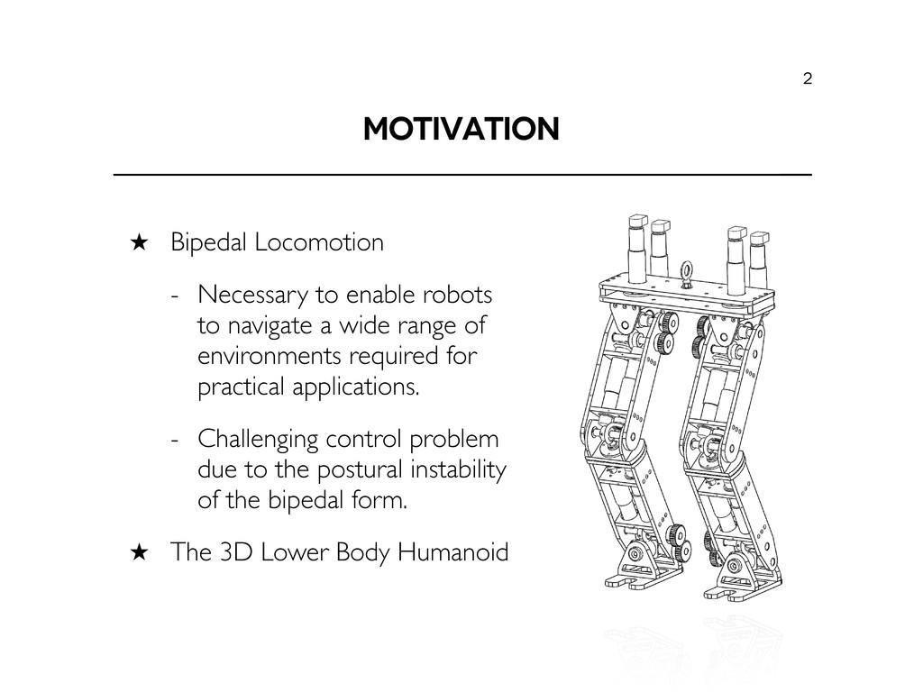
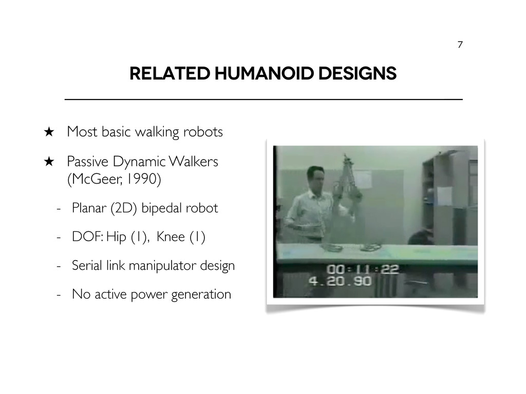
navigate a wide range of environments required for practical applications. - Challenging control problem due to the postural instability of the bipedal form. ˒ The 3D Lower Body Humanoid 2
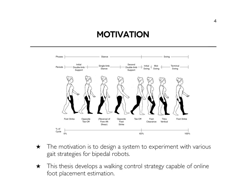
experiment with various gait strategies for bipedal robots. ˒ This thesis develops a walking control strategy capable of online foot placement estimation. 4
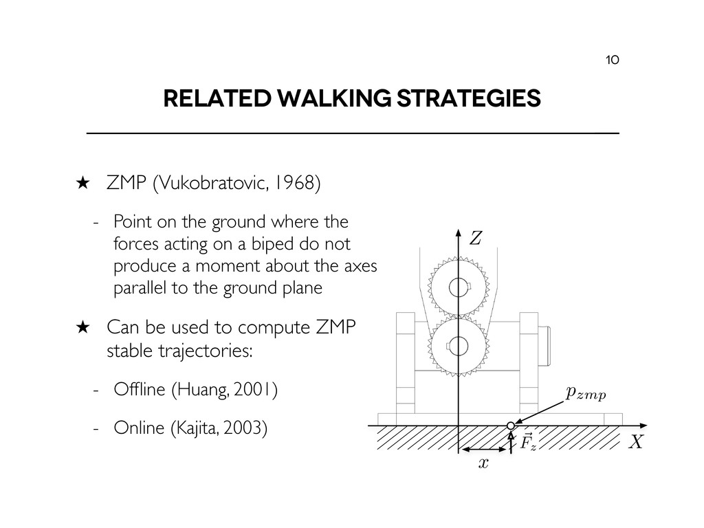
(Vukobratovic, 1968) - Point on the ground where the forces acting on a biped do not produce a moment about the axes parallel to the ground plane ˒ Can be used to compute ZMP stable trajectories: - Offline (Huang, 2001) - Online (Kajita, 2003) 10
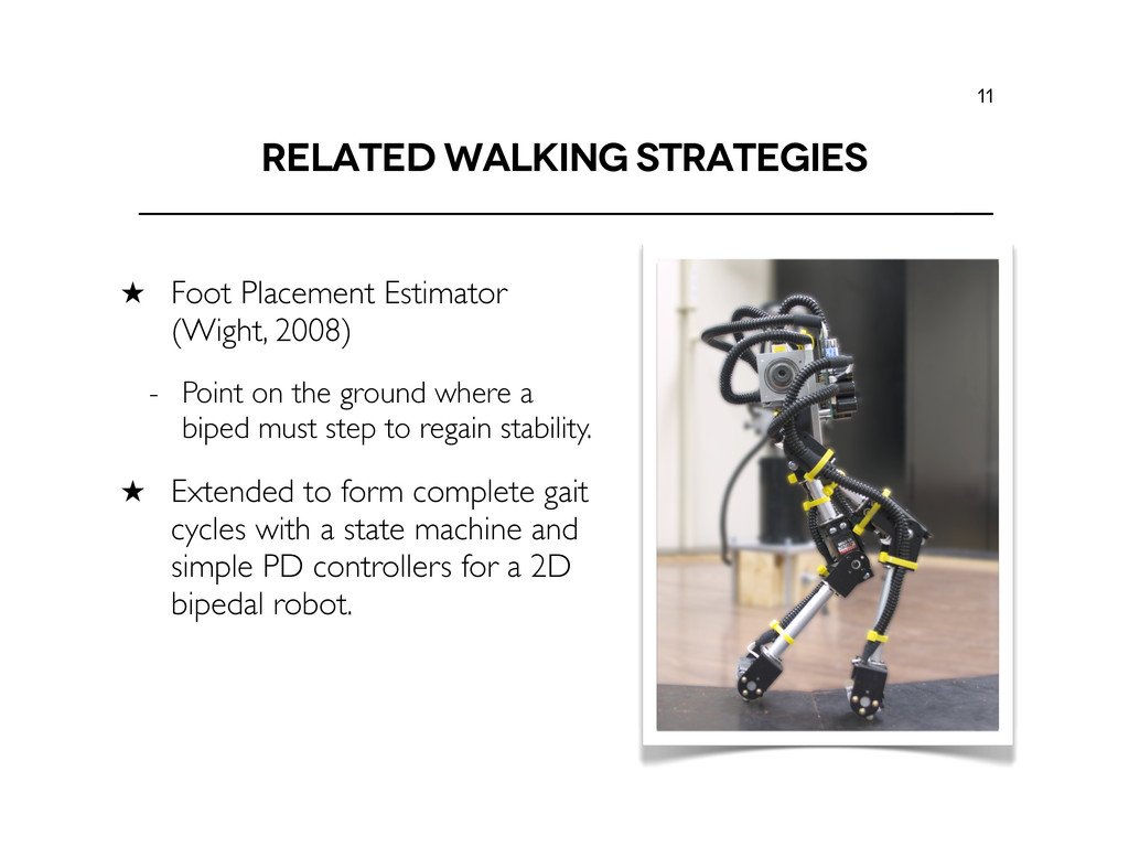
Point on the ground where a biped must step to regain stability. ˒ Extended to form complete gait cycles with a state machine and simple PD controllers for a 2D bipedal robot. 11
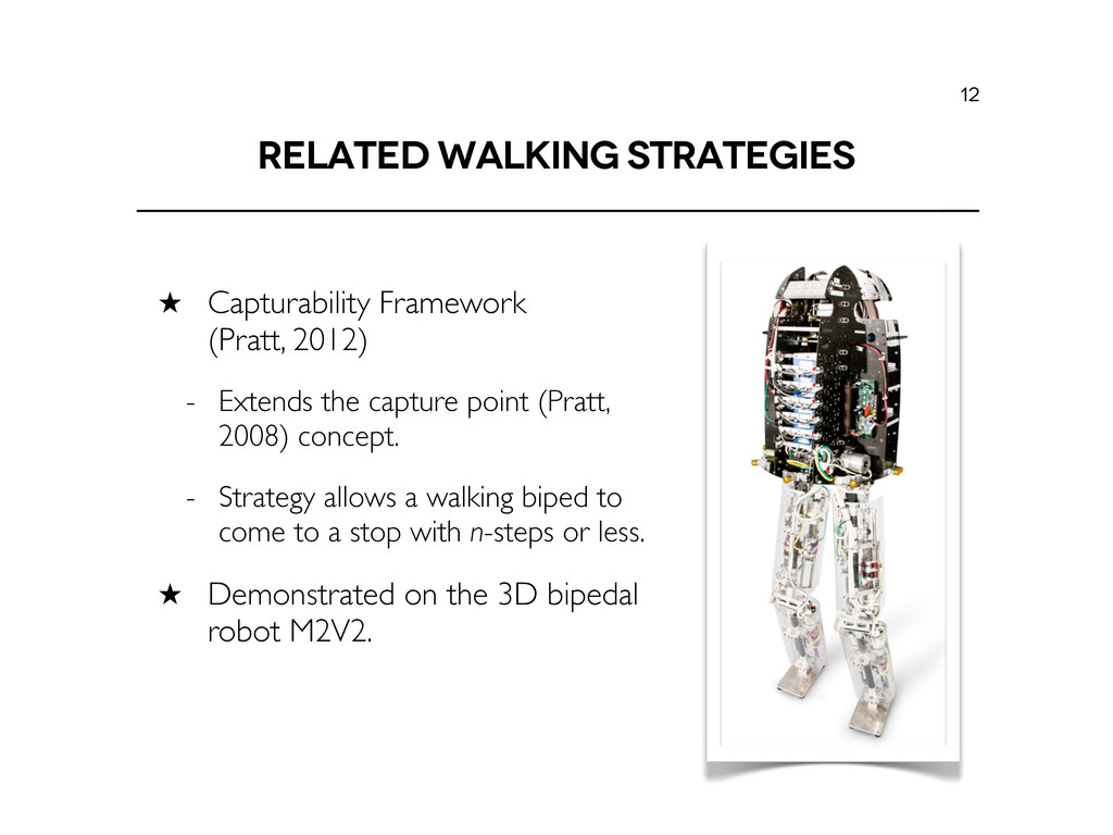
the capture point (Pratt, 2008) concept. - Strategy allows a walking biped to come to a stop with n-steps or less. ˒ Demonstrated on the 3D bipedal robot M2V2. 12
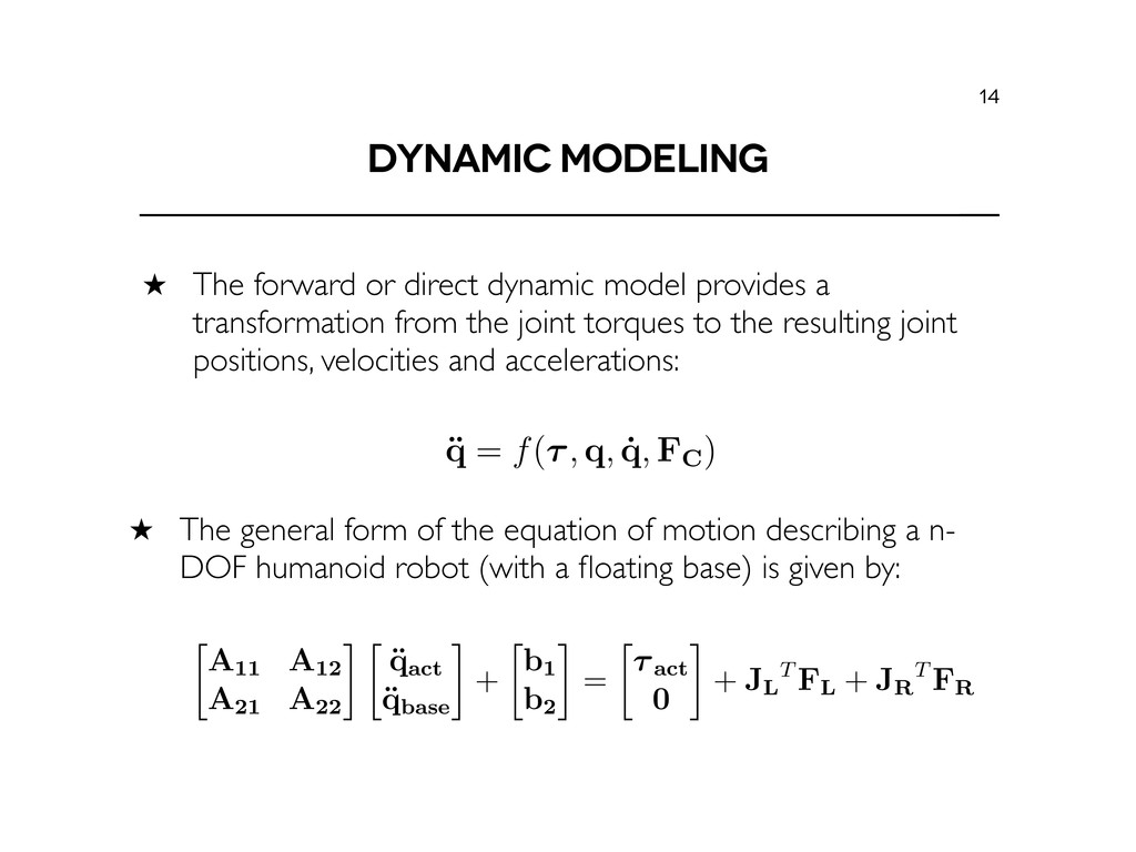
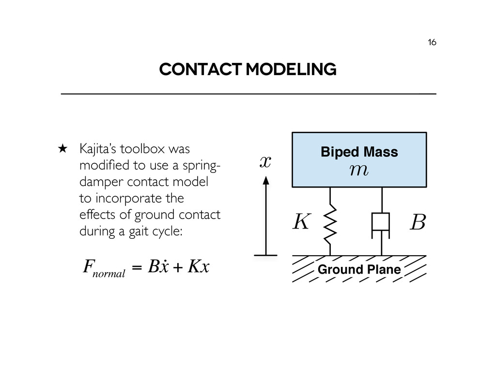
a transformation from the joint torques to the resulting joint positions, velocities and accelerations: 14 Dynamic Modeling namic model of the proposed system must be developed and analyzed under ting conditions to determine the forces acting on the system and torques expe h of the joints. The forward or direct dynamic model provides a transformati int torques (⌧) to the resulting joint positions (q), velocities (˙ q) and accele ¨ q = f(⌧, q, ˙ q, FC ) presents the contact force(s) felt at the feet. Given this model, a dynamic sim onment can be designed to estimate the torque loading at di↵erent joints al robot during the gait cycle. This estimate can form the basis of the initia fications from which motors and gearing can be selected. An important consid s model is the inclusion of contact forces during the stance phase of the gai ground reaction forces exerted on the robots feet have a significant impact mic requirements of each joint. ˒ The general form of the equation of motion describing a n- DOF humanoid robot (with a floating base) is given by: Where A(q) is the (n + 6) ⇥ (n + 6) inertia matrix, C(q, ˙ q) are the centripetal/Cor rms, g(q) is the gravity vector and J is the Jacobian matrix which provides the mapp etween the joint and work space variables. The (n + 6) ⇥ 1 generalized force vector gmented as follows: ⌧ = ⇥⌧act ⌧base ⇤T ( Where ⌧act represents the n actuated DOF and ⌧base = 06⇥1 are the remaining n tuated DOF at the floating base. In order to incorporate the e↵ects of contact force oth feet of the biped robot, (3.2) is expanded as follows: A11 A12 A21 A22 ¨ qact ¨ qbase + b1 b2 = ⌧act 0 + JL T FL + JR T FR ( Where the generalized acceleration vector ¨ qact represents the n-DOF joint motion and ¨ q presents the 6 DOF base motion. The gravitational and Coriolis terms are combi to the b vector. The J and J are 6 x n Jacobian matrices for the left and r
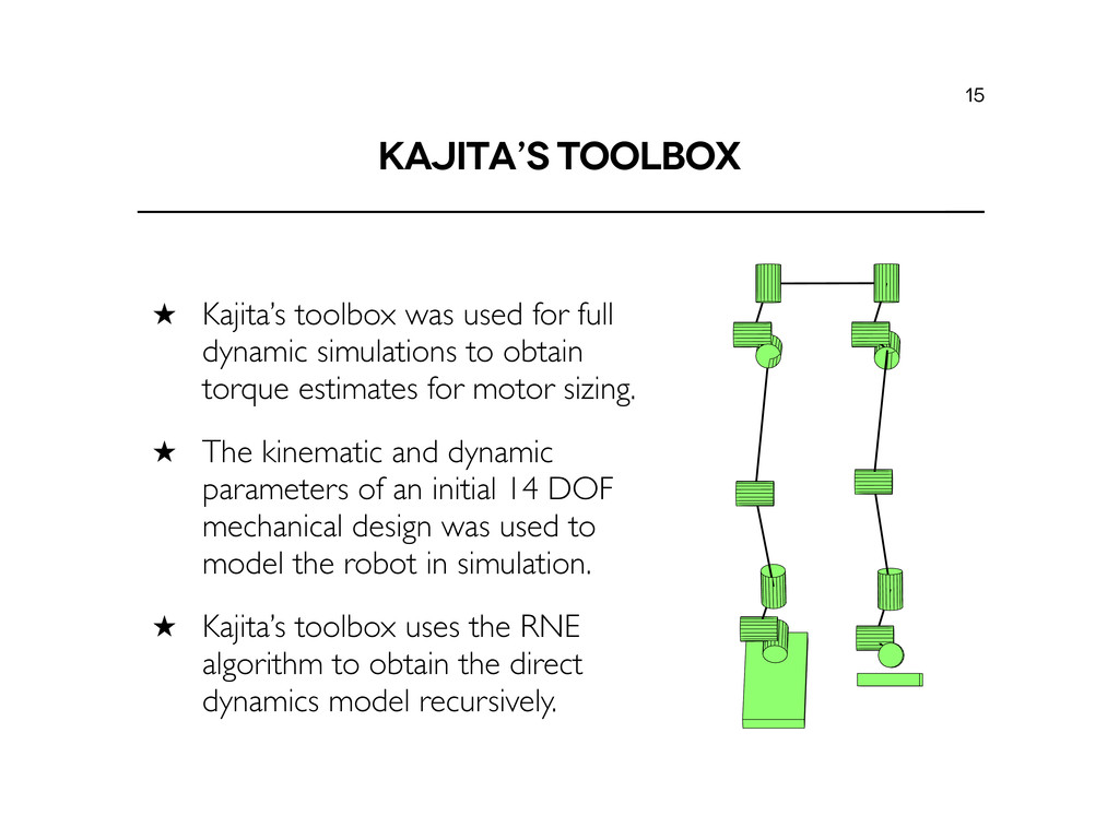
simulations to obtain torque estimates for motor sizing. ˒ The kinematic and dynamic parameters of an initial 14 DOF mechanical design was used to model the robot in simulation. ˒ Kajita’s toolbox uses the RNE algorithm to obtain the direct dynamics model recursively. 15
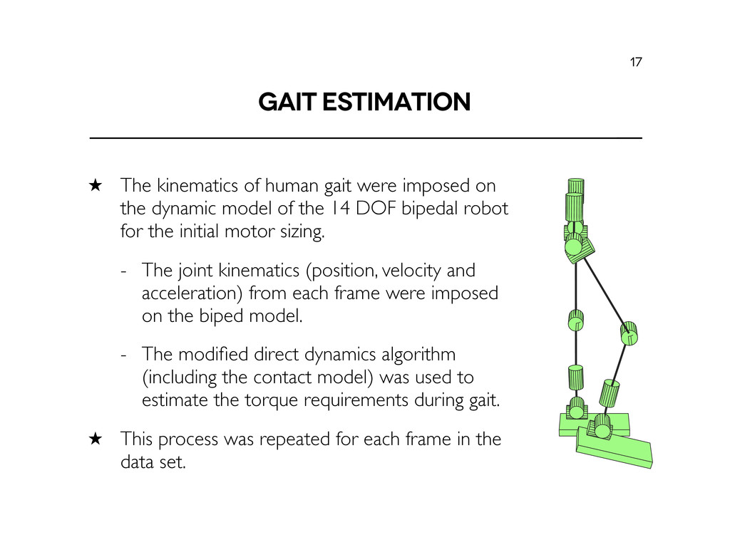
on the dynamic model of the 14 DOF bipedal robot for the initial motor sizing. - The joint kinematics (position, velocity and acceleration) from each frame were imposed on the biped model. - The modified direct dynamics algorithm (including the contact model) was used to estimate the torque requirements during gait. ˒ This process was repeated for each frame in the data set. 17
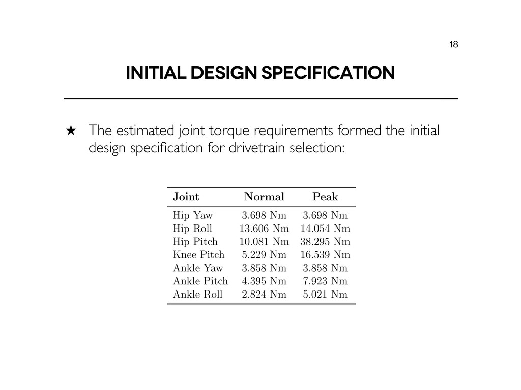
the initial design specification for drivetrain selection: 18 Table 3.2: Individual joint torque demands for each DOF in one leg using gait estimation. Joint Normal Peak Hip Yaw 3.698 Nm 3.698 Nm Hip Roll 13.606 Nm 14.054 Nm Hip Pitch 10.081 Nm 38.295 Nm Knee Pitch 5.229 Nm 16.539 Nm Ankle Yaw 3.858 Nm 3.858 Nm Ankle Pitch 4.395 Nm 7.923 Nm Ankle Roll 2.824 Nm 5.021 Nm di↵erent models selected from the manufacturer and it also simplifies the electromechanical design process. The combined initial design specifications for the drivetrain components are summarized in Table 3.3. For the initial design, the normal torque specification is obtained by taking an average of joint torque values during the swing phase. Since the ground reaction forces experienced during the stance phase produce large torques in a short
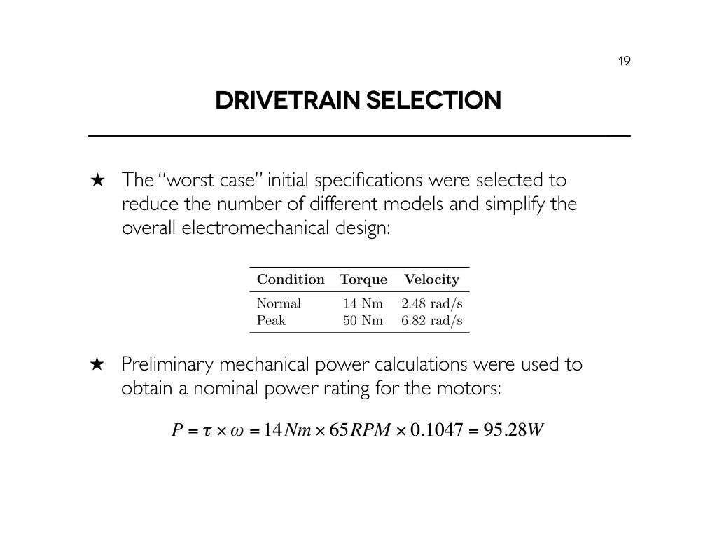
to reduce the number of different models and simplify the overall electromechanical design: 19 Hip Pitch 10.081 Nm 38.295 Nm Knee Pitch 5.229 Nm 16.539 Nm Ankle Yaw 3.858 Nm 3.858 Nm Ankle Pitch 4.395 Nm 7.923 Nm Ankle Roll 2.824 Nm 5.021 Nm di↵erent models selected from the manufacturer and it also simplifies the electromechanical design process. The combined initial design specifications for the drivetrain components are summarized in Table 3.3. For the initial design, the normal torque specification is obtained by taking an average of joint torque values during the swing phase. Since the ground reaction forces experienced during the stance phase produce large torques in a short period of time, the peak torque specification is obtained by selecting the highest torque value from all frames. Table 3.3: Initial design specifications for drivetrain components. Condition Torque Velocity Normal 14 Nm 2.48 rad/s Peak 50 Nm 6.82 rad/s The contact model parameters (spring and damping coe cients) were observed to have a noticeable e↵ect on the peak design specifications. Since the contact model only provides a crude approximation of the ground reaction forces that the real robot will experience, the final selected value was chosen to provide a peak torque which averages between the largest and smallest values. The final spring and damping coe cients used in deriving the design specifications were K = 10000 and B = 100, respectively. ˒ Preliminary mechanical power calculations were used to obtain a nominal power rating for the motors: P = τ ×ω = 14Nm × 65RPM × 0.1047 = 95.28W
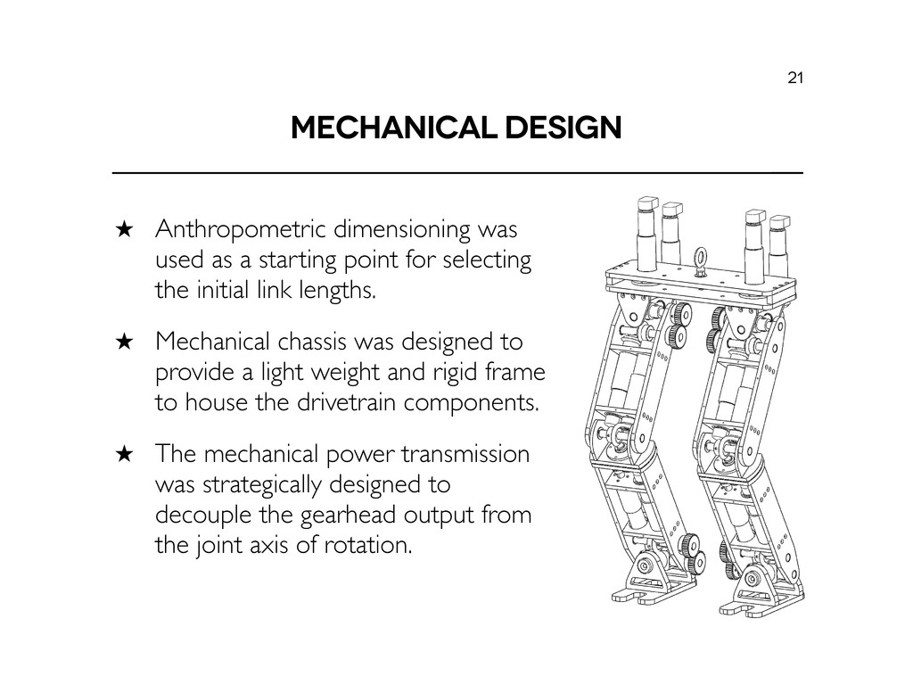
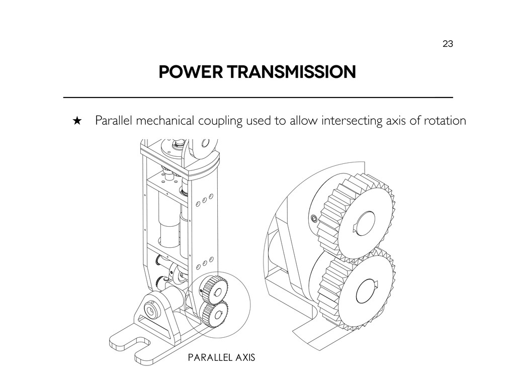
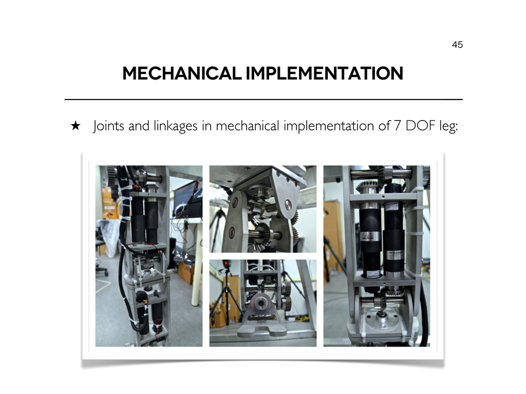
point for selecting the initial link lengths. ˒ Mechanical chassis was designed to provide a light weight and rigid frame to house the drivetrain components. ˒ The mechanical power transmission was strategically designed to decouple the gearhead output from the joint axis of rotation. 21
robotic systems is an iterative process: - Starts from a mechanical model in CAD software. - Parameters are transferred to a dynamic simulator for analysis. - Design is revised in CAD to improve the performance. ˒ Process is repeated until the mechanical design achieves some desired goal. 25
iterations of robotic and mechatronic systems, consisting of: - A native add-in for the CAD package SolidWorks that exports a model for simulation - Model generation counter part in Matlab/Simulink to recreate the CAD equivalent model ˒ The entire process is semi-automated and requires minimal user input. 26
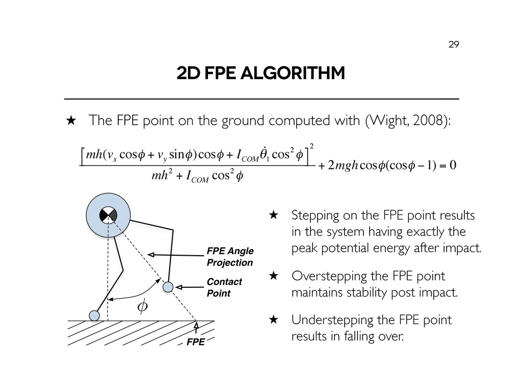
computed with (Wight, 2008): 29 φ FPE Contact Point FPE Angle Projection mh(v x cosφ + v y sinφ)cosφ + I COM θ1 cos2 φ ⎡ ⎣ ⎤ ⎦ 2 mh2 + I COM cos2 φ + 2mghcosφ(cosφ −1) = 0 ˒ Stepping on the FPE point results in the system having exactly the peak potential energy after impact. ˒ Overstepping the FPE point maintains stability post impact. ˒ Understepping the FPE point results in falling over.
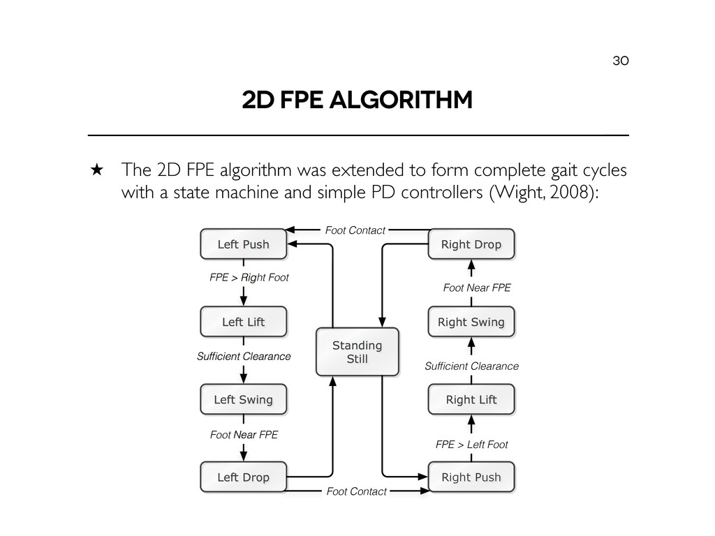
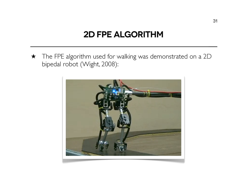
to form complete gait cycles with a state machine and simple PD controllers (Wight, 2008): 30 Standing Still Left Push Left Lift Left Swing Left Drop FPE > Right Foot Sufficient Clearance Foot Near FPE Right Drop Right Swing Right Lift Right Push Foot Near FPE Sufficient Clearance FPE > Left Foot Foot Contact Foot Contact
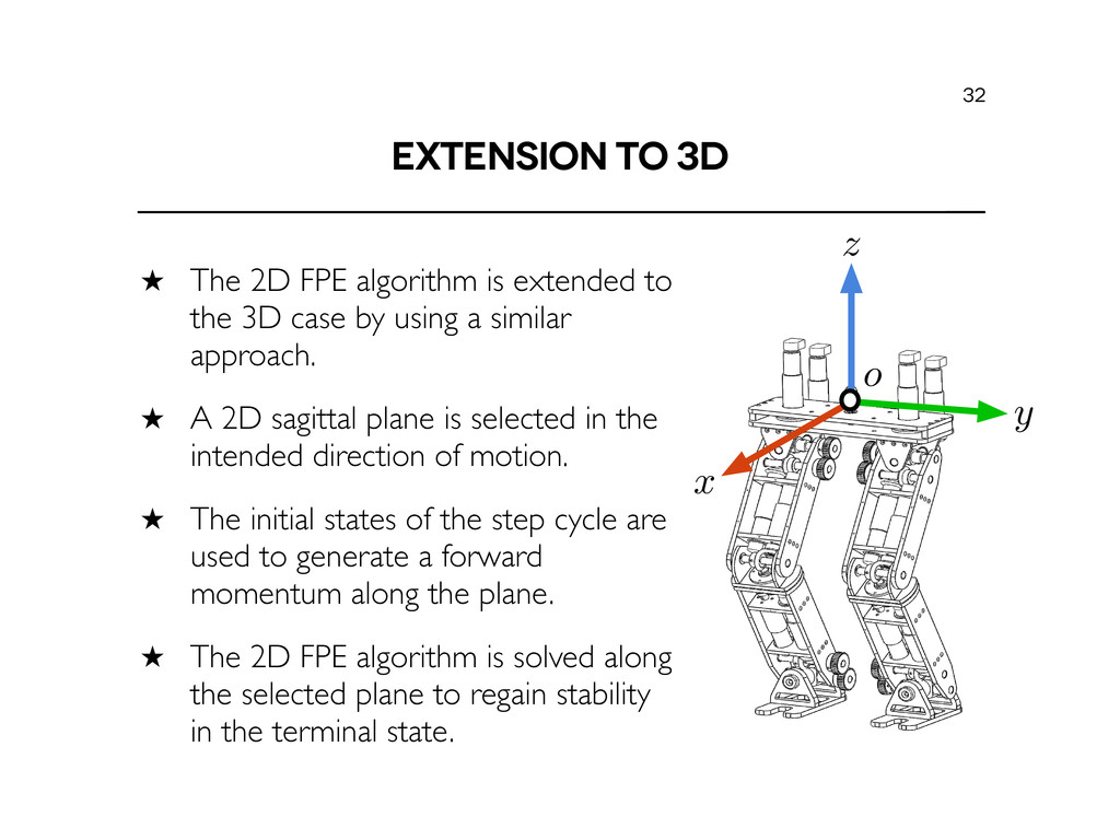
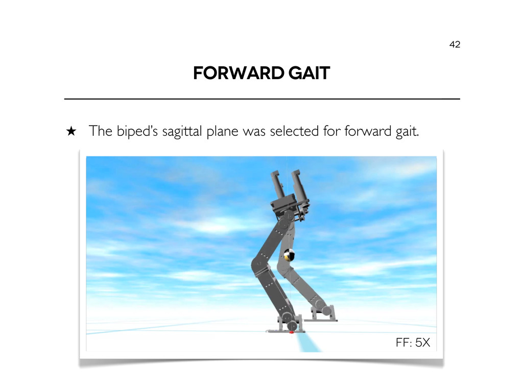
to the 3D case by using a similar approach. ˒ A 2D sagittal plane is selected in the intended direction of motion. ˒ The initial states of the step cycle are used to generate a forward momentum along the plane. ˒ The 2D FPE algorithm is solved along the selected plane to regain stability in the terminal state. 32 x y z o
swing foot to initiate the gait sequence. ˒ The generated trajectories must simultaneously ensure that: - A forward momentum is generated along the selected plane. - Off-sagittal stability is maintained while the momentum is generated. 34
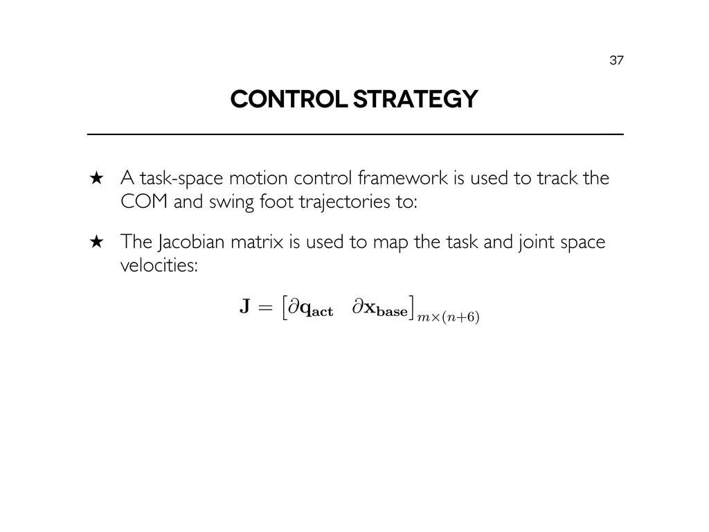
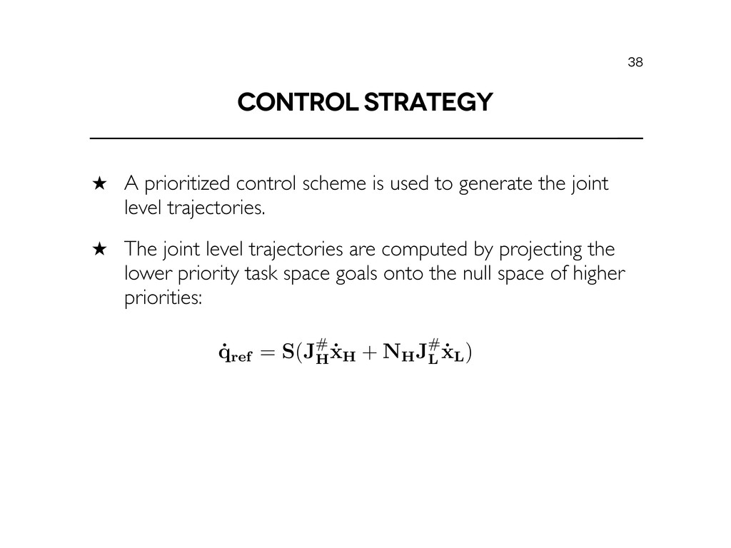
to track the COM and swing foot trajectories to: ˒ The Jacobian matrix is used to map the task and joint space velocities: 37 ybrid control strategy is used to simultaneously maintain stability in the o↵-sag ne, achieve su cient forward momentum along a selected sagittal plane and ultim k the FPE location to regain stability by taking a step. Similar to the appr sented in [7], this approach uses a state machine to transition through the step sequ h each state having a local controller. ing the initial states of the step cycle, whole body motion control is used to trac OM and xSWING trajectories described in Section 5.1.2. To generate the correspon t level trajectories, the Jacobian matrix is used to map between the task space an t space velocities: J = ⇥@qact @xbase ⇤ m⇥(n+6) rioritized task space control scheme is used to generate joint level trajectories w ultaneously achieve state goals while satisfying the highest priority constraint (i.e. the xCOM position). The state-dependent joint level trajectories can be compute jecting the lower priority task space goals onto the null space of higher priorities: ˙ qref = S(J# H ˙ xH + NH J# L ˙ xL )
generate the joint level trajectories. ˒ The joint level trajectories are computed by projecting the lower priority task space goals onto the null space of higher priorities: 38 M and xSWING trajectories described in Section 5.1.2. To generate the correspon level trajectories, the Jacobian matrix is used to map between the task space and space velocities: J = ⇥@qact @xbase ⇤ m⇥(n+6) ( ioritized task space control scheme is used to generate joint level trajectories w ltaneously achieve state goals while satisfying the highest priority constraint (i.e. h he xCOM position). The state-dependent joint level trajectories can be computed ecting the lower priority task space goals onto the null space of higher priorities: ˙ qref = S(J# H ˙ xH + NH J# L ˙ xL ) ( 69
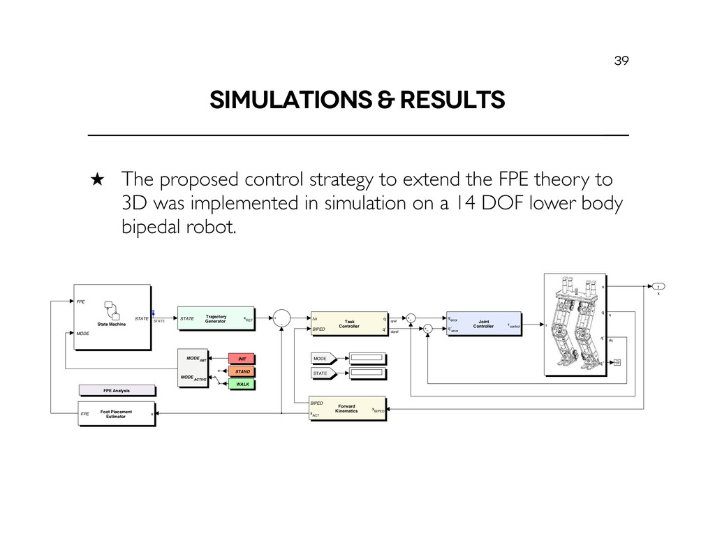
the FPE theory to 3D was implemented in simulation on a 14 DOF lower body bipedal robot. 39 x 1 MODE INIT MODE ACTIVE WALK Trajectory Generator STATE x REF Task Controller BIPED Δx q q" State Machine MODE FPE STATE STAND τ x q q" q"" Joint Controller q error q" error τ control INIT Forward Kinematics x BIPED BIPED x ACT FPE Analysis STATE MODE Foot Placement Estimator x FPE q dq dqref qref STATE
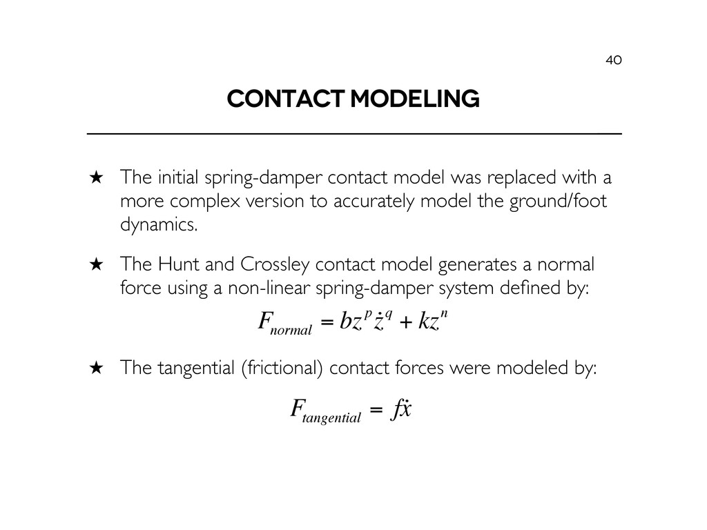
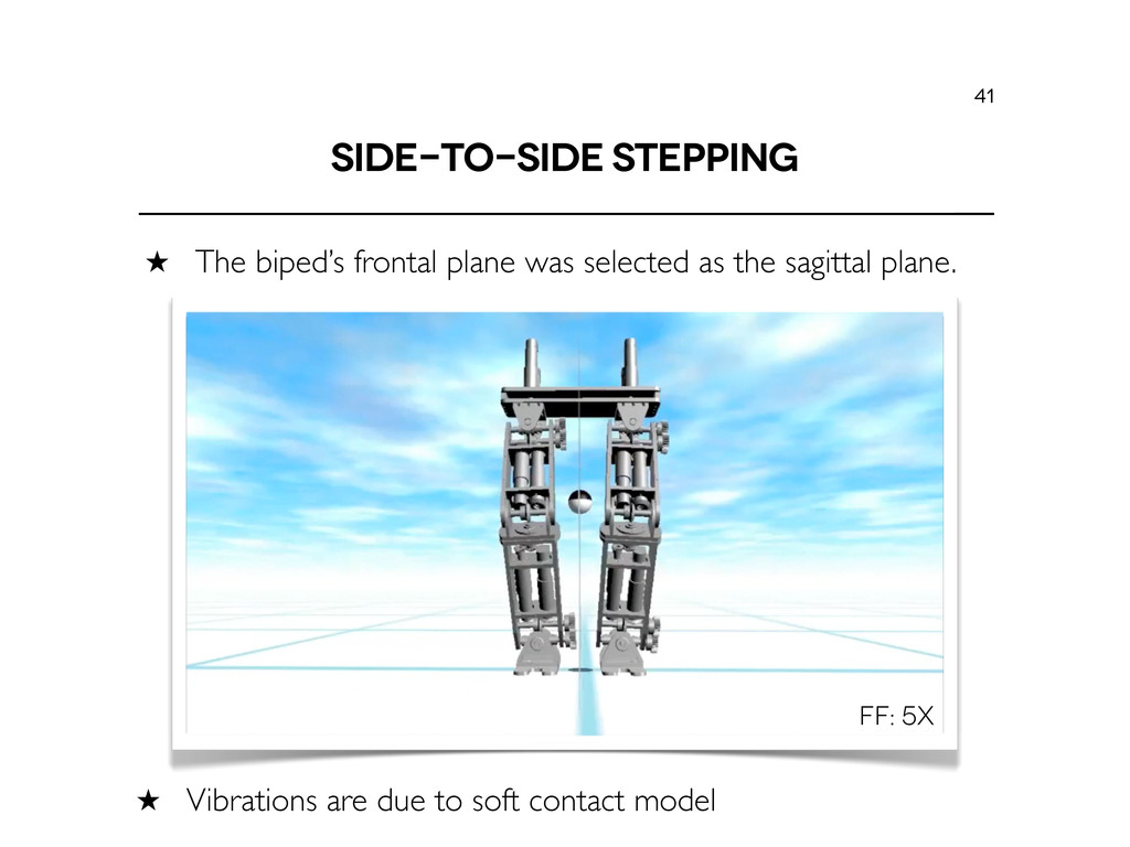
with a more complex version to accurately model the ground/foot dynamics. ˒ The Hunt and Crossley contact model generates a normal force using a non-linear spring-damper system defined by: ˒ The tangential (frictional) contact forces were modeled by: 40 F normal = bzp zq + kzn F tangential = f x
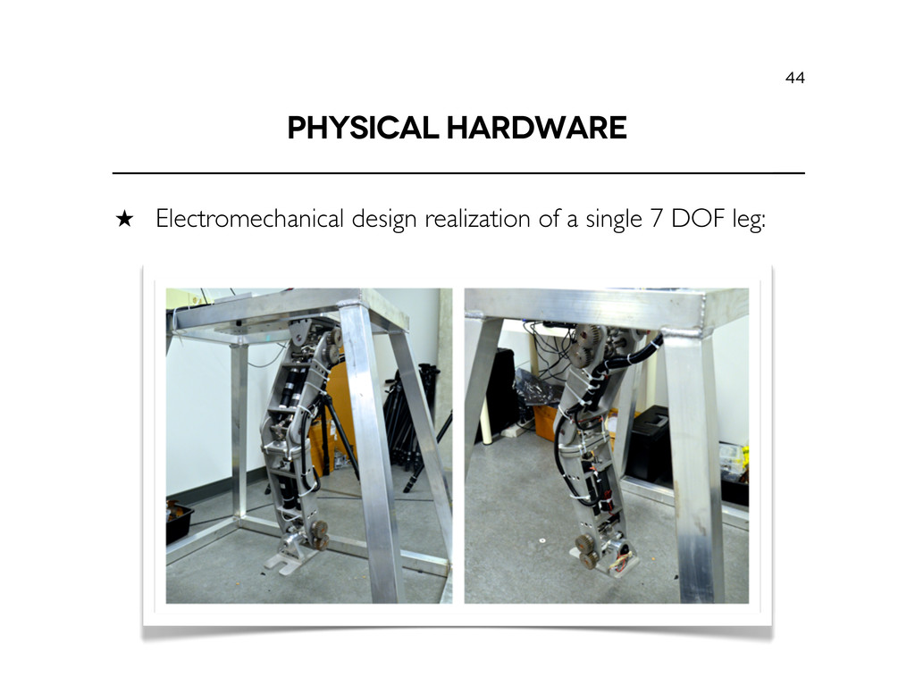
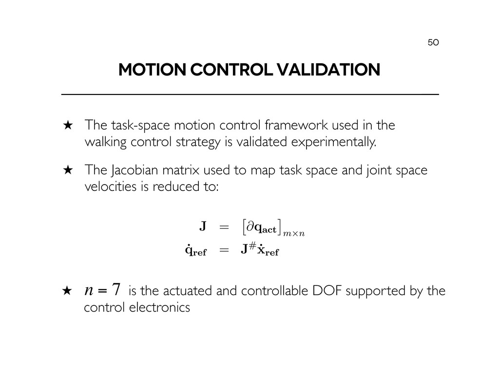
in the walking control strategy is validated experimentally. ˒ The Jacobian matrix used to map task space and joint space velocities is reduced to: 50 .5 Motion Control Validation his section describes the experiments validating the motion control framework in Sec on 5.1.3 using the HIL environment. The parallel model concept was extended to develo gher level task space controllers to generate the joint level trajectories for simulation an rdware. The interim control electronics provided by Quanser Inc are limited to contro ng 7 DOF simultaneously. Therefore, only a single 7 DOF bipedal robot leg wired t e control electronics was used for the experiments in this section. The biped’s torso wa gidly attached to the supporting frame in the fixed configuration, removing the 6 unac ated DOF. The Jacobian matrix used to map the task space and joint space velocitie (5.1) is reduced to: J = ⇥@qact ⇤ m⇥n (6.11 ˙ qref = J# ˙ xref (6.12 here n = 7 is the actuated and controllable DOF supported by the control electronics he joint level commands are generated from the task space trajectories (˙ xref ) using (6.12) ternatively, the prioritized task space control scheme in Section 5.1.3 can be used to s ultaneously satisfy high priority constraints. The mapping provided by (5.2) is simplifie removing the actuator selection matrix S, since there are no unactuated DOF. ˒ is the actuated and controllable DOF supported by the control electronics n = 7
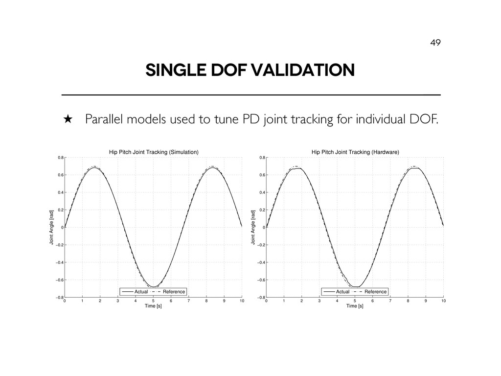
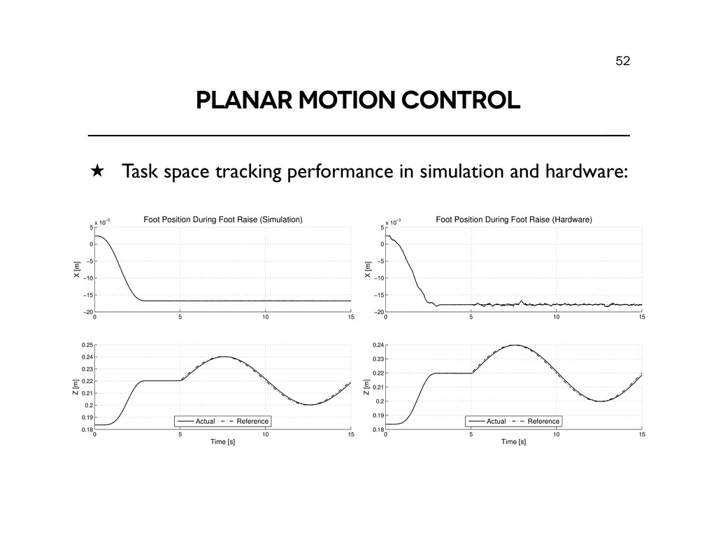
and hardware: 52 controller. The gains were tuned in simulation to achieve the desired tracking performance before attempting the experiment on the physical hardware. The foot position tracking using KP = 10 and KD = 0.1 is shown in Figure 6.13 in simulation and on hardware. The trajectory on the physical hardware along the x direction is not as smooth as its simulated counterpart. Unmodeled backlash in the pitch joints (i.e. the knee) is the cause behind this di↵erence. However, the PD control gains in the task space and joint space controllers are high enough to achieve the desired tracking performance. The experimental results demonstrate the simplified version of the motion control frame- work with n = 3 DOF. The pitch joint trajectories are automatically generated from the desired swing foot height and the resulting motion bends the knee joint as the foot is raised. 0 5 10 15 −20 −15 −10 −5 0 5 x 10⁻³ Foot Position During Foot Raise (Simulation) X [m] 0 5 10 15 0.18 0.19 0.2 0.21 0.22 0.23 0.24 0.25 Z [m] Time [s] Actual Reference 0 5 10 15 −20 −15 −10 −5 0 5 x 10⁻³ Foot Position During Foot Raise (Hardware) X [m] 0 5 10 15 0.18 0.19 0.2 0.21 0.22 0.23 0.24 Z [m] Time [s] Actual Reference Figure 6.13: Task space trajectory tracking for bending the knee and raising the leg in simulation and hardware.
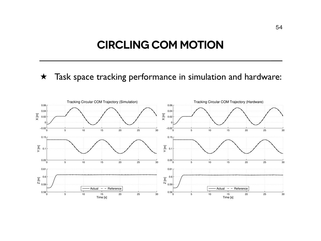
and hardware: 54 0 5 10 15 20 25 30 −0.02 0 0.02 0.04 0.06 Tracking Circular COM Trajectory (Simulation) X [m] 0 5 10 15 20 25 30 0.05 0.1 0.15 Y [m] 0 5 10 15 20 25 30 0.58 0.59 0.6 0.61 Z [m] Time [s] Actual Reference 0 5 10 15 20 25 30 −0.02 0 0.02 0.04 0.06 Tracking Circular COM Trajectory (Hardware) X [m] 0 5 10 15 20 25 30 0.05 0.1 0.15 Y [m] 0 5 10 15 20 25 30 0.58 0.59 0.6 0.61 Z [m] Time [s] Actual Reference Figure 6.18: Task space tracking of circular COM motion in software and hardware. ˙ xCOM represents the cartesian position of the foot in the world frame. The tracking results
the physical platform. ˒ Rapid prototyping toolchain developed to streamline the design process of complex multibody systems. ˒ Gait synthesis through the extension of the FPE algorithm for 3D bipedal robots. ˒ Experimental validation of key components of the proposed walking control strategy. 55