Constraint Composite Graph-Based Lifted Message Passing for Distributed Constraint Optimization Problems

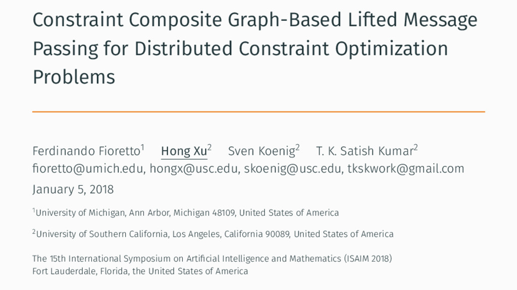
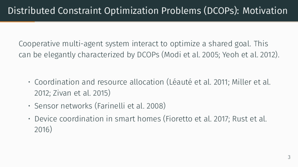
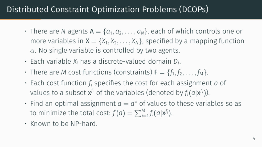
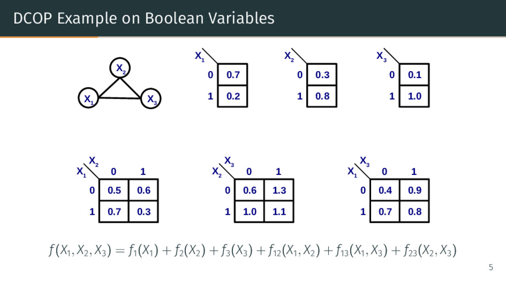
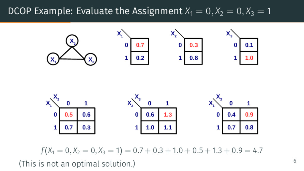
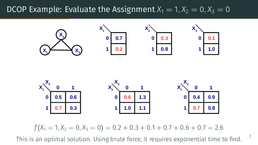
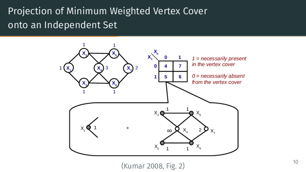
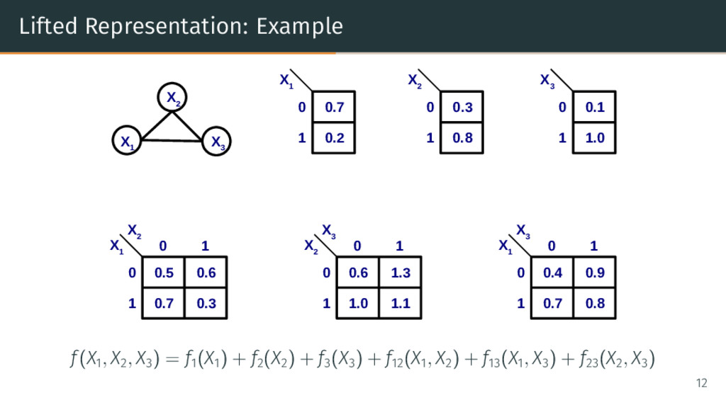
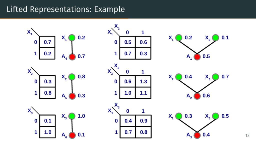
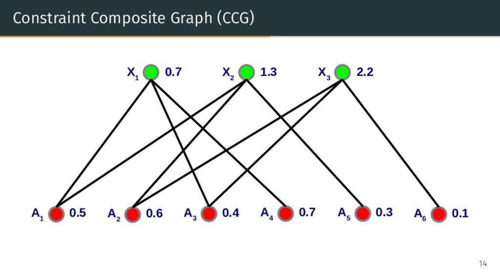
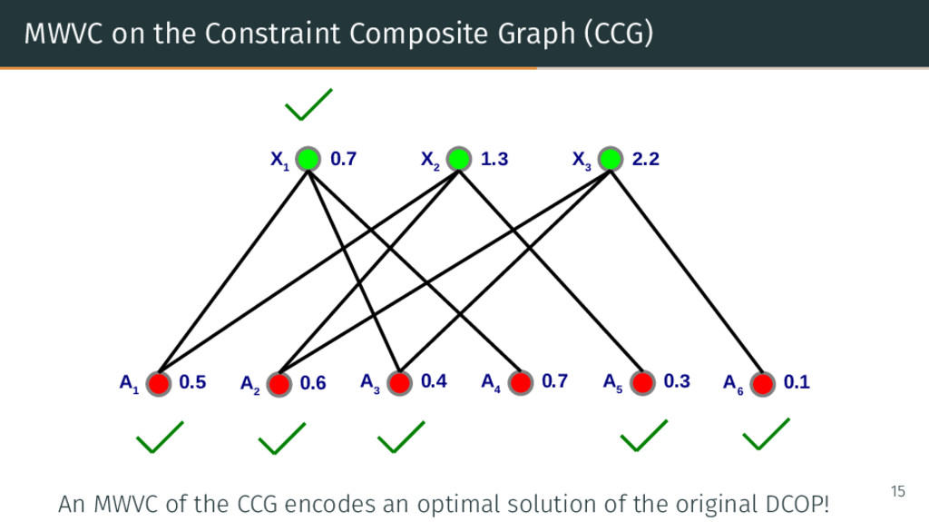
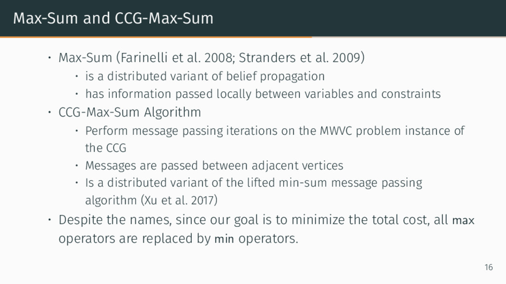
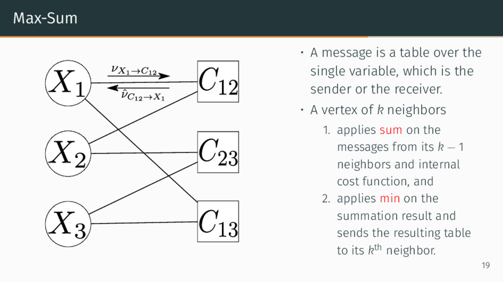
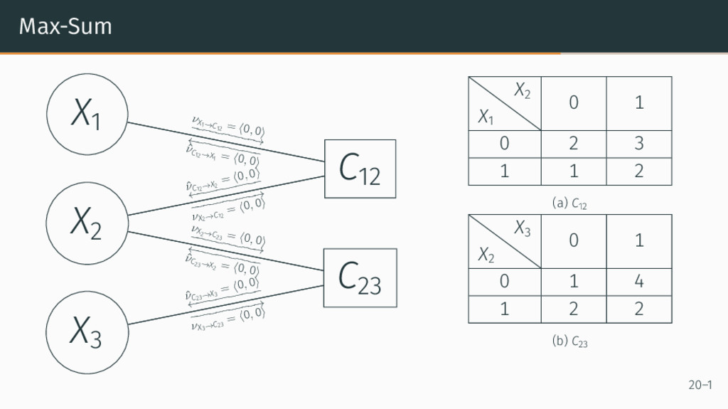
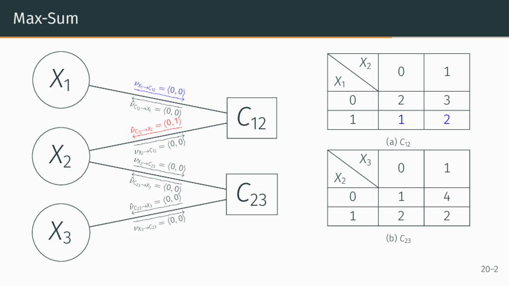
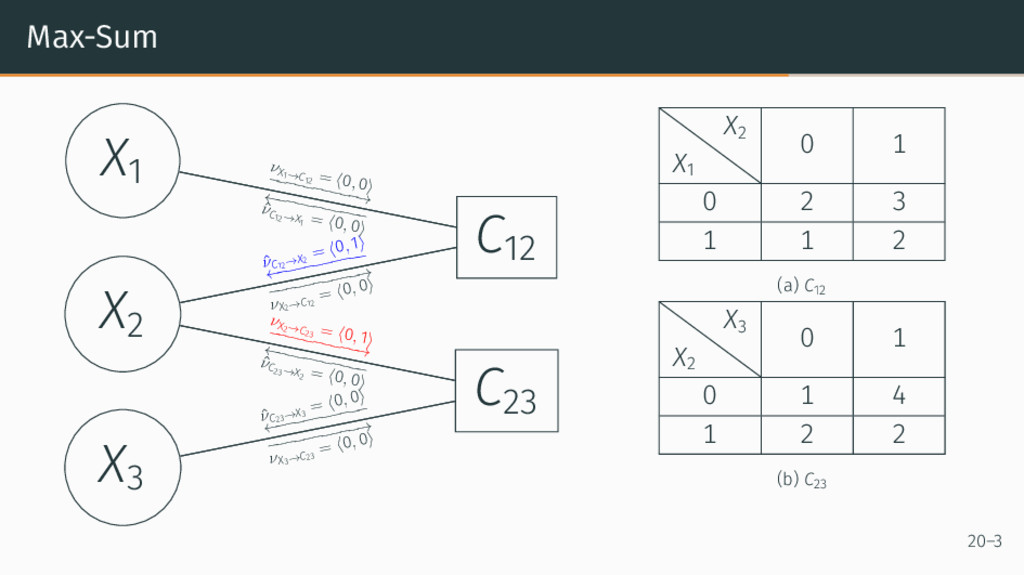
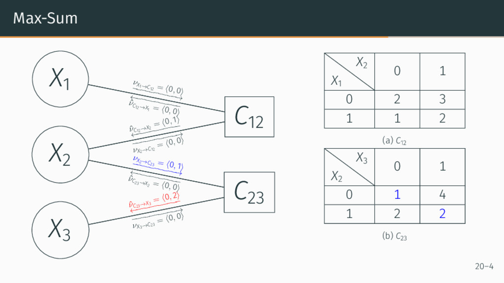
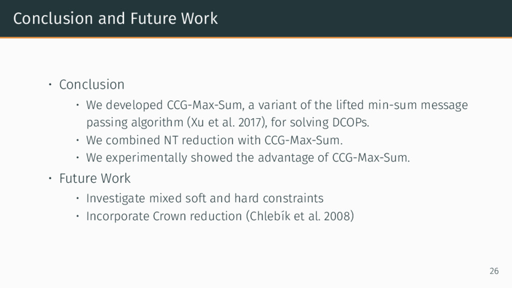
The presentation slides of the paper "Ferdinando Fioretto, Hong Xu, Sven Koenig, and T. K. Satish Kumar. Constraint composite graph-based lifted message passing for distributed constraint optimization problems. In Proceedings of the 15th International Symposium on Artificial Intelligence and Mathematics (ISAIM). 2018."

More details: http://www.hong.me/papers/fioretto2018.html
Link to published paper: http://isaim2018.cs.virginia.edu/papers/ISAIM2018_Fioretto_etal.pdf

Transcript

1. Constraint Composite Graph-Based Lifted Message Passing for Distributed Constraint Optimization Problems Ferdinando Fioretto1 Hong Xu2 Sven Koenig2 T. K. Satish Kumar2 fioretto@umich.edu, hongx@usc.edu, skoenig@usc.edu, tkskwork@gmail.com January 5, 2018 1University of Michigan, Ann Arbor, Michigan 48109, United States of America 2University of Southern California, Los Angeles, California 90089, United States of America The 15th International Symposium on Artificial Intelligence and Mathematics (ISAIM 2018) Fort Lauderdale, Florida, the United States of America
2. Summary For solving distributed constraint optimization problems (DCOPs), we develop CCG-Max-Sum, a distributed variant of the lifted min-sum message passing algorithm (Xu et al. 2017) based on the Constraint Composite Graph (Kumar 2008). We experimentally showed that CCG-Max-Sum outperformed other competitors. 1
3. Agenda Distributed Constraint Optimization Problems (DCOPs) The Constraint Composite Graph (CCG) CCG-Max-Sum Max-Sum and CCG-Max-Sum The Nemhauser-Trotter (NT) Reduction Experimental Evaluation Conclusion and Future Work 2
4. Agenda Distributed Constraint Optimization Problems (DCOPs) The Constraint Composite Graph (CCG) CCG-Max-Sum Max-Sum and CCG-Max-Sum The Nemhauser-Trotter (NT) Reduction Experimental Evaluation Conclusion and Future Work
5. Distributed Constraint Optimization Problems (DCOPs): Motivation Cooperative multi-agent system interact to optimize a shared goal. This can be elegantly characterized by DCOPs (Modi et al. 2005; Yeoh et al. 2012). • Coordination and resource allocation (Léauté et al. 2011; Miller et al. 2012; Zivan et al. 2015) • Sensor networks (Farinelli et al. 2008) • Device coordination in smart homes (Fioretto et al. 2017; Rust et al. 2016) 3
6. Distributed Constraint Optimization Problems (DCOPs) • There are N agents A = {a1 , a2 , . . . , aN }, each of which controls one or more variables in X = {X1 , X2 , . . . , XN }, specified by a mapping function α. No single variable is controlled by two agents. • Each variable Xi has a discrete-valued domain Di . • There are M cost functions (constraints) F = {f1 , f2 , . . . , fM }. • Each cost function fi specifies the cost for each assignment a of values to a subset xfi of the variables (denoted by fi (a|xfi )). • Find an optimal assignment a = a∗ of values to these variables so as to minimize the total cost: f(a) = M i=1 fi (a|xfi ). • Known to be NP-hard. 4
7. DCOP Example on Boolean Variables X 1 X 2 X 3 X 2 1 0 1 0 X 3 1.0 0.6 1.3 1.1 X 1 1 0 1 0 X 3 0.7 0.4 0.9 0.8 X 1 1 0 1 0 X 2 0.7 0.5 0.6 0.3 X 1 1 0 0.2 0.7 X 3 1 0 1.0 0.1 X 2 1 0 0.8 0.3 f(X1 , X2 , X3 ) = f1 (X1 ) + f2 (X2 ) + f3 (X3 ) + f12 (X1 , X2 ) + f13 (X1 , X3 ) + f23 (X2 , X3 ) 5
8. DCOP Example: Evaluate the Assignment X1 = 0, X2 = 0, X3 = 1 X 1 X 2 X 3 X 2 1 0 1 0 X 3 1.0 0.6 1.3 1.1 X 1 1 0 1 0 X 3 0.7 0.4 0.9 0.8 X 1 1 0 1 0 X 2 0.7 0.5 0.6 0.3 X 1 1 0 0.2 0.7 X 3 1 0 1.0 0.1 X 2 1 0 0.8 0.3 f(X1 = 0, X2 = 0, X3 = 1) = 0.7 + 0.3 + 1.0 + 0.5 + 1.3 + 0.9 = 4.7 (This is not an optimal solution.) 6
9. DCOP Example: Evaluate the Assignment X1 = 1, X2 = 0, X3 = 0 X 1 X 2 X 3 X 2 1 0 1 0 X 3 1.0 0.6 1.3 1.1 X 1 1 0 1 0 X 3 0.7 0.4 0.9 0.8 X 1 1 0 1 0 X 2 0.7 0.5 0.6 0.3 X 1 1 0 0.2 0.7 X 3 1 0 1.0 0.1 X 2 1 0 0.8 0.3 f(X1 = 1, X2 = 0, X3 = 0) = 0.2 + 0.3 + 0.1 + 0.7 + 0.6 + 0.7 = 2.6 This is an optimal solution. Using brute force, it requires exponential time to find. 7
10. Agenda Distributed Constraint Optimization Problems (DCOPs) The Constraint Composite Graph (CCG) CCG-Max-Sum Max-Sum and CCG-Max-Sum The Nemhauser-Trotter (NT) Reduction Experimental Evaluation Conclusion and Future Work
11. Two Forms of Structure in DCOPs X 1 X 2 X 3 X 4 X 1 1 0 1 0 X 2 0.7 0.5 0.6 0.3 Numerical Structure Graphical Structure • Graphical: Which variables are in which cost functions? • Numerical: How does each cost function relate the variables in it? How can we exploit both forms of structure computationally? 8
12. Minimum Weighted Vertex Cover (MWVC) 1 2 2 0 1 1 (a)  1 2 2 0 1 1 (b)  1 2 2 0 1 1 (c)  1 2 2 0 1 1 (d)  Each vertex is associated with a non-negative weight. Sum of the weights on the vertices in the vertex cover is minimized. 9
13. Projection of Minimum Weighted Vertex Cover onto an Independent Set X 1 + X 3 X 2 X 5 X 6 X 4 X 7 ∞ 1 1 1 1 2 1 X 1 X 2 X 3 X 4 X 5 X 6 X 7 1 1 1 1 2 3 1 = necessarily present in the vertex cover 0 = necessarily absent from the vertex cover X 1 1 0 1 0 X 4 5 4 7 6 1 (Kumar 2008, Fig. 2) 10
14. Projection of MWVC onto an Independent Set Assuming Boolean variables in DCOPs • Observation: The projection of MWVC onto an independent set looks similar to a cost function. • Question 1: Can we build the lifted graphical representation for any given cost function? This is answered by (Kumar 2008). • Question 2: What is the benefit of doing so? 11
15. Lifted Representation: Example X 1 X 2 X 3 X 2 1 0 1 0 X 3 1.0 0.6 1.3 1.1 X 1 1 0 1 0 X 3 0.7 0.4 0.9 0.8 X 1 1 0 1 0 X 2 0.7 0.5 0.6 0.3 X 1 1 0 0.2 0.7 X 3 1 0 1.0 0.1 X 2 1 0 0.8 0.3 f(X1 , X2 , X3 ) = f1 (X1 ) + f2 (X2 ) + f3 (X3 ) + f12 (X1 , X2 ) + f13 (X1 , X3 ) + f23 (X2 , X3 ) 12
16. Lifted Representations: Example X 2 1 0 1 0 X 3 1.0 0.6 1.3 1.1 X 1 1 0 1 0 X 3 0.7 0.4 0.9 0.8 X 1 1 0 1 0 0.7 0.5 0.6 0.3 X 1 1 0 0.2 0.7 X 3 1 0 1.0 0.1 X 2 1 0 0.8 0.3 X 1 A 4 0.2 0.7 X 2 A 5 0.8 0.3 X 3 A 6 1.0 0.1 X 1 A 1 0.2 0.5 X 2 0.1 X 2 A 2 0.4 0.6 X 3 0.7 X 1 A 3 0.3 0.4 X 3 0.5 X 2 13
17. Constraint Composite Graph (CCG) X 1 A 1 0.7 0.5 X 2 1.3 A 2 0.6 X 3 2.2 A 3 0.4 A 4 0.7 A 5 0.3 A 6 0.1 14
18. MWVC on the Constraint Composite Graph (CCG) X 1 A 1 0.7 0.5 X 2 1.3 A 2 0.6 X 3 2.2 A 3 0.4 A 4 0.7 A 5 0.3 A 6 0.1 An MWVC of the CCG encodes an optimal solution of the original DCOP! 15
19. Agenda Distributed Constraint Optimization Problems (DCOPs) The Constraint Composite Graph (CCG) CCG-Max-Sum Max-Sum and CCG-Max-Sum The Nemhauser-Trotter (NT) Reduction Experimental Evaluation Conclusion and Future Work
20. Agenda Distributed Constraint Optimization Problems (DCOPs) The Constraint Composite Graph (CCG) CCG-Max-Sum Max-Sum and CCG-Max-Sum The Nemhauser-Trotter (NT) Reduction Experimental Evaluation Conclusion and Future Work
21. Max-Sum and CCG-Max-Sum • Max-Sum (Farinelli et al. 2008; Stranders et al. 2009) • is a distributed variant of belief propagation • has information passed locally between variables and constraints • CCG-Max-Sum Algorithm • Perform message passing iterations on the MWVC problem instance of the CCG • Messages are passed between adjacent vertices • Is a distributed variant of the lifted min-sum message passing algorithm (Xu et al. 2017) • Despite the names, since our goal is to minimize the total cost, all max operators are replaced by min operators. 16
22. Operations on Tables: Min minX1 X1 X2 0 1 0 1 2 1 4 3 = X1 0 1 1 3 17
23. Operations on Tables: Sum X1 X2 0 1 0 1 2 1 4 3 + X1 0 5 1 6 = X1 X2 0 1 0 1 + 5 = 6 2 + 5 = 7 1 4 + 6 = 10 3 + 6 = 9 18
24. Max-Sum • A message is a table over the single variable, which is the sender or the receiver. • A vertex of k neighbors 1. applies sum on the messages from its k − 1 neighbors and internal cost function, and 2. applies min on the summation result and sends the resulting table to its kth neighbor. 19
25. Max-Sum X1 C12 X2 C23 X3 νX1→C12 = 0, 0 − − − − − − − − − − → − − − − − − − − − − → νX3 →C23 = 0, 0 ˆ νC12 →X2 = 0, 0 ← − − − − − − − − − − νX2→C23 = 0, 0 − − − − − − − − − − → ˆ νC23 →X3 = 0, 0 ← − − − − − − − − − − ← − − − − − − − − − − ˆ νC23→X2 = 0, 0 − − − − − − − − − − → νX2 →C12 = 0, 0 ← − − − − − − − − − − ˆ νC12→X1 = 0, 0 X1 X2 0 1 0 2 3 1 1 2 (a) C12 X2 X3 0 1 0 1 4 1 2 2 (b) C23 20–1
26. Max-Sum X1 C12 X2 C23 X3 νX1→C12 = 0, 0 − − − − − − − − − − → − − − − − − − − − − → νX3 →C23 = 0, 0 ˆ νC12 →X2 = 0, 1 ← − − − − − − − − − − νX2→C23 = 0, 0 − − − − − − − − − − → ˆ νC23 →X3 = 0, 0 ← − − − − − − − − − − ← − − − − − − − − − − ˆ νC23→X2 = 0, 0 − − − − − − − − − − → νX2 →C12 = 0, 0 ← − − − − − − − − − − ˆ νC12→X1 = 0, 0 X1 X2 0 1 0 2 3 1 1 2 (a) C12 X2 X3 0 1 0 1 4 1 2 2 (b) C23 20–2
27. Max-Sum X1 C12 X2 C23 X3 νX1→C12 = 0, 0 − − − − − − − − − − → − − − − − − − − − − → νX3 →C23 = 0, 0 ˆ νC12 →X2 = 0, 1 ← − − − − − − − − − − νX2→C23 = 0, 1 − − − − − − − − − − → ˆ νC23 →X3 = 0, 0 ← − − − − − − − − − − ← − − − − − − − − − − ˆ νC23→X2 = 0, 0 − − − − − − − − − − → νX2 →C12 = 0, 0 ← − − − − − − − − − − ˆ νC12→X1 = 0, 0 X1 X2 0 1 0 2 3 1 1 2 (a) C12 X2 X3 0 1 0 1 4 1 2 2 (b) C23 20–3
28. Max-Sum X1 C12 X2 C23 X3 νX1→C12 = 0, 0 − − − − − − − − − − → − − − − − − − − − − → νX3 →C23 = 0, 0 ˆ νC12 →X2 = 0, 1 ← − − − − − − − − − − νX2→C23 = 0, 1 − − − − − − − − − − → ˆ νC23 →X3 = 0, 2 ← − − − − − − − − − − ← − − − − − − − − − − ˆ νC23→X2 = 0, 0 − − − − − − − − − − → νX2 →C12 = 0, 0 ← − − − − − − − − − − ˆ νC12→X1 = 0, 0 X1 X2 0 1 0 2 3 1 1 2 (a) C12 X2 X3 0 1 0 1 4 1 2 2 (b) C23 20–4
29. Max-Sum X1 C12 X2 C23 X3 νX1→C12 = 0, 0 − − − − − − − − − − → − − − − − − − − − − → νX3 →C23 = 0, 0 ˆ νC12 →X2 = 0, 1 ← − − − − − − − − − − νX2→C23 = 0, 1 − − − − − − − − − − → ˆ νC23 →X3 = 0, 2 ← − − − − − − − − − − ← − − − − − − − − − − ˆ νC23→X2 = 0, 1 − − − − − − − − − − → νX2 →C12 = 0, 0 ← − − − − − − − − − − ˆ νC12→X1 = 0, 0 X1 X2 0 1 0 2 3 1 1 2 (a) C12 X2 X3 0 1 0 1 4 1 2 2 (b) C23 20–5
30. Max-Sum X1 C12 X2 C23 X3 νX1→C12 = 0, 0 − − − − − − − − − − → − − − − − − − − − − → νX3 →C23 = 0, 0 ˆ νC12 →X2 = 0, 1 ← − − − − − − − − − − νX2→C23 = 0, 1 − − − − − − − − − − → ˆ νC23 →X3 = 0, 2 ← − − − − − − − − − − ← − − − − − − − − − − ˆ νC23→X2 = 0, 1 − − − − − − − − − − → νX2 →C12 = 0, 1 ← − − − − − − − − − − ˆ νC12→X1 = 0, 0 X1 X2 0 1 0 2 3 1 1 2 (a) C12 X2 X3 0 1 0 1 4 1 2 2 (b) C23 20–6
31. Max-Sum X1 C12 X2 C23 X3 νX1→C12 = 0, 0 − − − − − − − − − − → − − − − − − − − − − → νX3 →C23 = 0, 0 ˆ νC12 →X2 = 0, 1 ← − − − − − − − − − − νX2→C23 = 0, 1 − − − − − − − − − − → ˆ νC23 →X3 = 0, 2 ← − − − − − − − − − − ← − − − − − − − − − − ˆ νC23→X2 = 0, 1 − − − − − − − − − − → νX2 →C12 = 0, 1 ← − − − − − − − − − − ˆ νC12→X1 = 1, 0 X1 X2 0 1 0 2 3 1 1 2 (a) C12 X2 X3 0 1 0 1 4 1 2 2 (b) C23 20–7
32. Max-Sum X1 C12 X2 C23 X3 νX1→C12 = 0, 0 − − − − − − − − − − → − − − − − − − − − − → νX3 →C23 = 0, 0 ˆ νC12 →X2 = 0, 1 ← − − − − − − − − − − νX2→C23 = 0, 1 − − − − − − − − − − → ˆ νC23 →X3 = 0, 2 ← − − − − − − − − − − ← − − − − − − − − − − ˆ νC23→X2 = 0, 1 − − − − − − − − − − → νX2 →C12 = 0, 1 ← − − − − − − − − − − ˆ νC12→X1 = 1, 0 • X1 = 1 minimizes ˆ νC12→X1 (X1 ) • X2 = 0 minimizes ˆ νC12→X2 (X2 ) + ˆ νC23→X2 (X2 ) • X3 = 0 minimizes ˆ νC23→X3 (X3 ) • Optimal solution: X1 = 1, X2 = 0, X3 = 0 20–8
33. CCG-Max-Sum: Finding an MWVC on the CCG • Treat MWVC problems on the CCG as DCOPs and apply Max-Sum on them. • Messages are simplified passed between adjacent vertices. µi u→v = max    wu − t∈N(u)\{v} µi−1 t→u , 0    , 21
34. Agenda Distributed Constraint Optimization Problems (DCOPs) The Constraint Composite Graph (CCG) CCG-Max-Sum Max-Sum and CCG-Max-Sum The Nemhauser-Trotter (NT) Reduction Experimental Evaluation Conclusion and Future Work
35. Motivation: Kernelization and the Nemhauser-Trotter Reduction • The MWVC problem is known to be NP-hard. • To solve such a problem, an algorithm that reduces the size of the problem in polynomial time is desirable. • A kernelization method is one such algorithm. • The Nemhauser-Trotter (NT) Reduction is one kernelization method for the MWVC problem. • The Constraint Composite Graph enables the use of the NT reduction. 22
36. The Nemhauser-Trotter (NT) Reduction A C D B w 4 w 3 w 1 w 2 A(w 1 ) B(w 2 ) C(w 3 ) D(w 4 ) A'(w 1 ) C'(w 3 ) D'(w 4 ) B'(w 2 ) A(w 1 ) B(w 2 ) C(w 3 ) D(w 4 ) A'(w 1 ) C'(w 3 ) D'(w 4 ) B'(w 2 ) A is in the minimum weighted VC B is not in the minimum weighted VC C and D are in the Kernel 23
37. Agenda Distributed Constraint Optimization Problems (DCOPs) The Constraint Composite Graph (CCG) CCG-Max-Sum Max-Sum and CCG-Max-Sum The Nemhauser-Trotter (NT) Reduction Experimental Evaluation Conclusion and Future Work
38. Experimental Setup • Algorithms • CCG-Max-Sum • CCG-Max-Sum-k: CCG-Max-Sum + NT reduction • Max-Sum (Farinelli et al. 2008; Stranders et al. 2009) • DSA (Zhang et al. 2005) • Benchmark instances • Grid networks (2-d 10 × 10 grids) • Scale-free networks (Barabási-Albert model (Barabási et al. 1999)), m = m0 = 2 • Random networks (Erdős-Rényi model (Erdős et al. 1959)), p1 = 0.4 and p1 = 0.8, max arity = 4 • 30 benchmark instances in each instance set, 100 agents/variables • Costs are uniformly random numbers from 1 to 100. 24
39. Max-Sum CCG-Max-Sum CCG-Max-Sum-k DSA 100 101 102 103 Iterations 6000 6500 7000 7500 8000 8500 9000 9500 Average Cost (a) grid networks 100 101 102 103 Iterations 7500 8000 8500 9000 9500 10000 10500 Average Cost (b) scale-free networks 100 101 102 103 Iterations 46000 47000 48000 49000 50000 Average Cost (c) low density random networks (p1 = 0.4) 100 101 102 103 Iterations 93000 94000 95000 96000 97000 98000 99000 100000 101000 Average Cost (d) high-density random networks (p1 = 0.8) 5,000 iterations for each benchmark instance. 25
40. Agenda Distributed Constraint Optimization Problems (DCOPs) The Constraint Composite Graph (CCG) CCG-Max-Sum Max-Sum and CCG-Max-Sum The Nemhauser-Trotter (NT) Reduction Experimental Evaluation Conclusion and Future Work
41. Conclusion and Future Work • Conclusion • We developed CCG-Max-Sum, a variant of the lifted min-sum message passing algorithm (Xu et al. 2017), for solving DCOPs. • We combined NT reduction with CCG-Max-Sum. • We experimentally showed the advantage of CCG-Max-Sum. • Future Work • Investigate mixed soft and hard constraints • Incorporate Crown reduction (Chlebík et al. 2008) 26
42. References I Albert-László Barabási and Réka Albert. “Emergence of Scaling in Random Networks”. In: Science 286.5439 (1999), pp. 509–512. Miroslav Chlebík and Janka Chlebíková. “Crown Reductions for the Minimum Weighted Vertex Cover Problem”. In: Discrete Applied Mathematics 156.3 (2008), pp. 292–312. P. Erdős and A. Rényi. “On Random Graphs I.”. In: Publicationes Mathematicae 6 (1959), pp. 290–297. Alessandro Farinelli, Alex Rogers, Adrian Petcu, and Nicholas Jennings. “Decentralised Coordination of Low-Power Embedded Devices Using the Max-Sum Algorithm”. In: Proceedings of the International Conference on Autonomous Agents and Multiagent Systems (AAMAS). 2008, pp. 639–646. Ferdinando Fioretto, William Yeoh, and Enrico Pontelli. “A Multiagent System Approach to Scheduling Devices in Smart Homes”. In: Proceedings of the International Conference on Autonomous Agents and Multiagent Systems (AAMAS). 2017, pp. 981–989.
43. References II T. K. Satish Kumar. “A Framework for Hybrid Tractability Results in Boolean Weighted Constraint Satisfaction Problems”. In: Proceedings of the International Conference on Principles and Practice of Constraint Programming (CP). 2008, pp. 282–297. Thomas Léauté and Boi Faltings. “Distributed Constraint Optimization Under Stochastic Uncertainty”. In: Proceedings of the AAAI Conference on Artificial Intelligence (AAAI). 2011, pp. 68–73. Sam Miller, Sarvapali D Ramchurn, and Alex Rogers. “Optimal decentralised dispatch of embedded generation in the smart grid”. In: Proceedings of the International Conference on Autonomous Agents and Multiagent Systems (AAMAS). 2012, pp. 281–288. Pragnesh Modi, Wei-Min Shen, Milind Tambe, and Makoto Yokoo. “ADOPT: Asynchronous Distributed Constraint Optimization with Quality Guarantees”. In: Artificial Intelligence 161.1–2 (2005), pp. 149–180. Pierre Rust, Gauthier Picard, and Fano Ramparany. “Using Message-Passing DCOP Algorithms to Solve Energy-Efficient Smart Environment Configuration Problems”. In: Proceedings of the International Joint Conference on Artificial Intelligence (IJCAI). 2016, pp. 468–474.
44. References III Ruben Stranders, Alessandro Farinelli, Alex Rogers, and Nick R Jennings. “Decentralised coordination of continuously valued control parameters using the Max-Sum algorithm”. In: Proceedings of the International Conference on Autonomous Agents and Multiagent Systems (AAMAS). 2009, pp. 601–608. Hong Xu, T. K. Satish Kumar, and Sven Koenig. “The Nemhauser-Trotter Reduction and Lifted Message Passing for the Weighted CSP”. In: Proceedings of the International Conference on Integration of Artificial Intelligence and Operations Research Techniques in Constraint Programming (CPAIOR). 2017, pp. 387–402. doi: 10.1007/978-3-319-59776-8_31. William Yeoh and Makoto Yokoo. “Distributed Problem Solving”. In: AI Magazine 33.3 (2012), pp. 53–65. Weixiong Zhang, Guandong Wang, Zhao Xing, and Lars Wittenberg. “Distributed Stochastic Search and Distributed Breakout: Properties, Comparison and Applications to Constraint Optimization Problems in Sensor Networks”. In: Artificial Intelligence 161.1–2 (2005), pp. 55–87.
45. References IV Roie Zivan, Harel Yedidsion, Steven Okamoto, Robin Glinton, and Katia Sycara. “Distributed Constraint Optimization for Teams of Mobile Sensing Agents”. In: Autonomous Agents and Multi-Agent Systems 29.3 (2015), pp. 495–536.