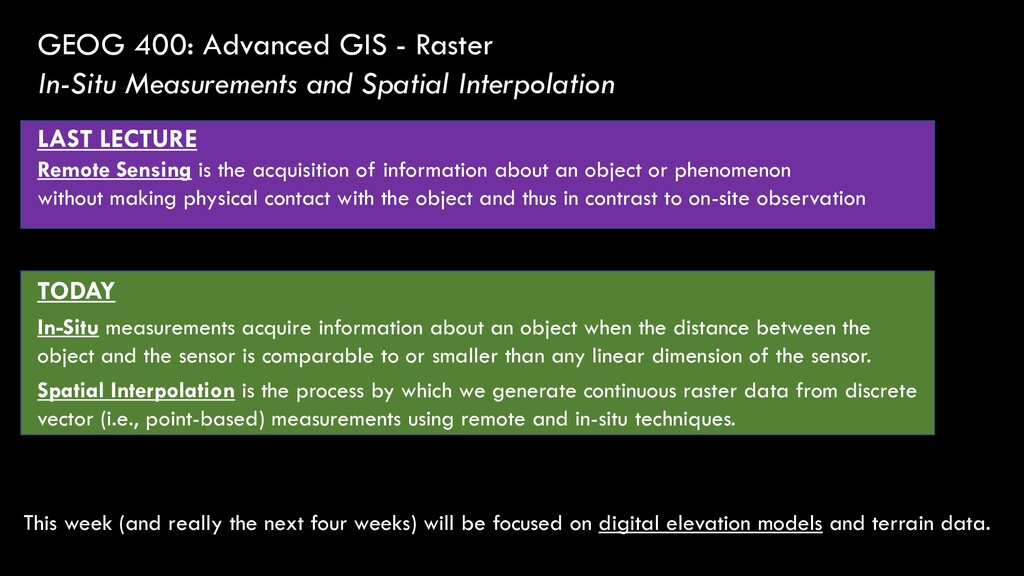
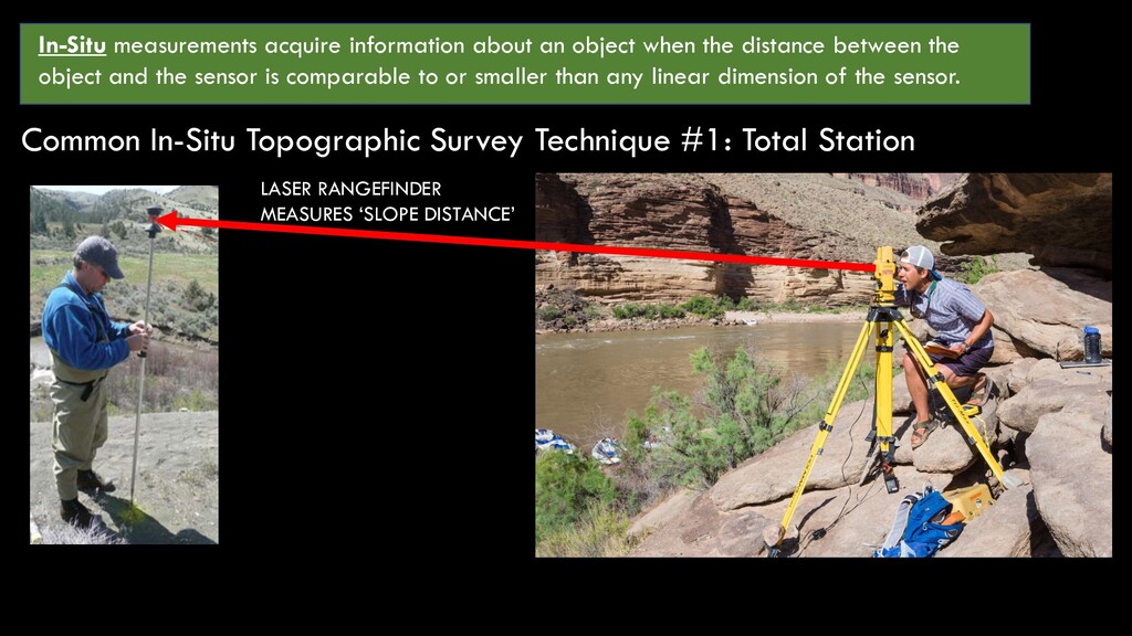
acquisition of information about an object or phenomenon without making physical contact with the object and thus in contrast to on-site observation In-Situ measurements acquire information about an object when the distance between the object and the sensor is comparable to or smaller than any linear dimension of the sensor. In-Situ Measurements and Spatial Interpolation Spatial Interpolation is the process by which we generate continuous raster data from discrete vector (i.e., point-based) measurements using remote and in-situ techniques. LAST LECTURE TODAY This week (and really the next four weeks) will be focused on digital elevation models and terrain data.
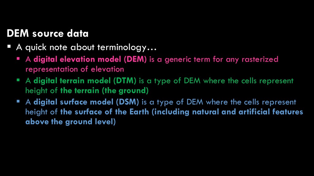
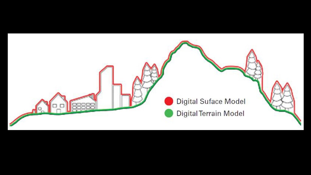
A digital elevation model (DEM) is a generic term for any rasterized representation of elevation ▪ A digital terrain model (DTM) is a type of DEM where the cells represent height of the terrain (the ground) ▪ A digital surface model (DSM) is a type of DEM where the cells represent height of the surface of the Earth (including natural and artificial features above the ground level)
between the object and the sensor is comparable to or smaller than any linear dimension of the sensor. Common In-Situ Topographic Survey Technique #1: Total Station LASER RANGEFINDER MEASURES ‘SLOPE DISTANCE’
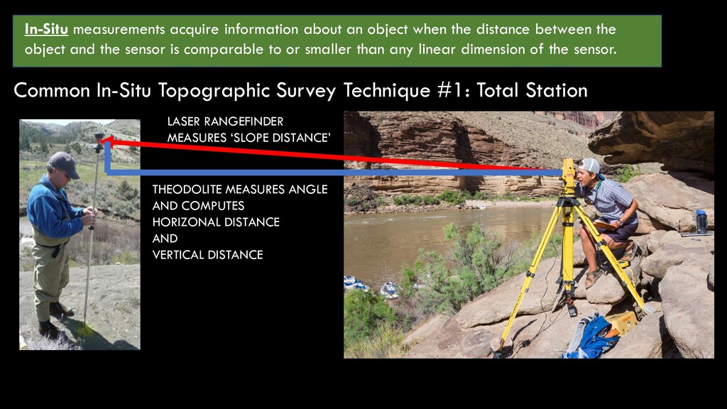
between the object and the sensor is comparable to or smaller than any linear dimension of the sensor. Common In-Situ Topographic Survey Technique #1: Total Station LASER RANGEFINDER MEASURES ‘SLOPE DISTANCE’ THEODOLITE MEASURES ANGLE AND COMPUTES HORIZONAL DISTANCE AND VERTICAL DISTANCE
between the object and the sensor is comparable to or smaller than any linear dimension of the sensor. Common In-Situ Topographic Survey Technique #1: Total Station LASER RANGEFINDER MEASURES ‘SLOPE DISTANCE’ THEODOLITE MEASURES ANGLE AND COMPUTES HORIZONAL DISTANCE AND VERTICAL DISTANCE Total station surveys generally require that we know where (exactly!) our instrument is set up
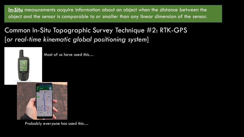
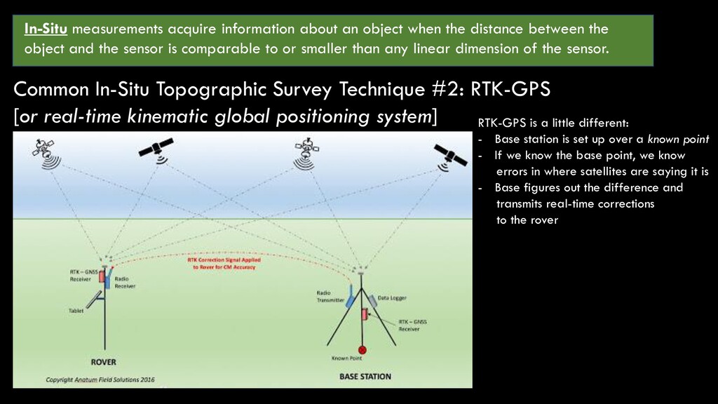
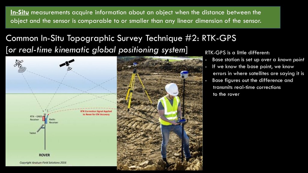
between the object and the sensor is comparable to or smaller than any linear dimension of the sensor. Common In-Situ Topographic Survey Technique #2: RTK-GPS [or real-time kinematic global positioning system] Most of us have used this… Probably everyone has used this…
between the object and the sensor is comparable to or smaller than any linear dimension of the sensor. Common In-Situ Topographic Survey Technique #2: RTK-GPS [or real-time kinematic global positioning system] Most of us have used this… Probably everyone has used this…
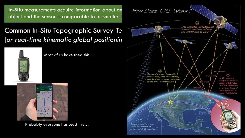
between the object and the sensor is comparable to or smaller than any linear dimension of the sensor. Common In-Situ Topographic Survey Technique #2: RTK-GPS [or real-time kinematic global positioning system] RTK-GPS is a little different: - Base station is set up over a known point - If we know the base point, we know errors in where satellites are saying it is - Base figures out the difference and transmits real-time corrections to the rover
between the object and the sensor is comparable to or smaller than any linear dimension of the sensor. Common In-Situ Topographic Survey Technique #2: RTK-GPS [or real-time kinematic global positioning system] RTK-GPS is a little different: - Base station is set up over a known point - If we know the base point, we know errors in where satellites are saying it is - Base figures out the difference and transmits real-time corrections to the rover
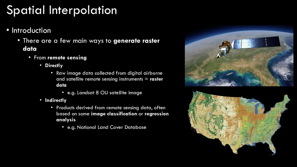
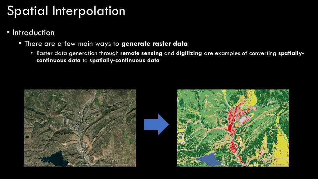
ways to generate raster data • From remote sensing • Directly • Raw image data collected from digital airborne and satellite remote sensing instruments = raster data • e.g. Landsat 8 OLI satellite image • Indirectly • Products derived from remote sensing data, often based on some image classification or regression analysis • e.g. National Land Cover Database
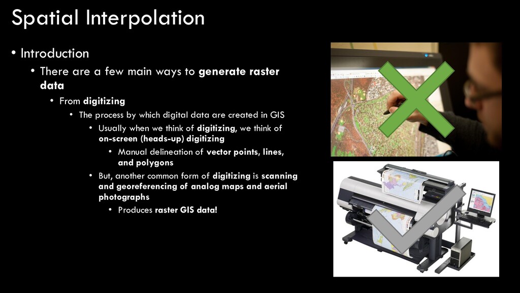
ways to generate raster data • From digitizing • The process by which digital data are created in GIS • Usually when we think of digitizing, we think of on-screen (heads-up) digitizing • Manual delineation of vector points, lines, and polygons • But, another common form of digitizing is scanning and georeferencing of analog maps and aerial photographs • Produces raster GIS data!
ways to generate raster data • Raster data generation through remote sensing and digitizing are examples of converting spatially- continuous data to spatially-continuous data
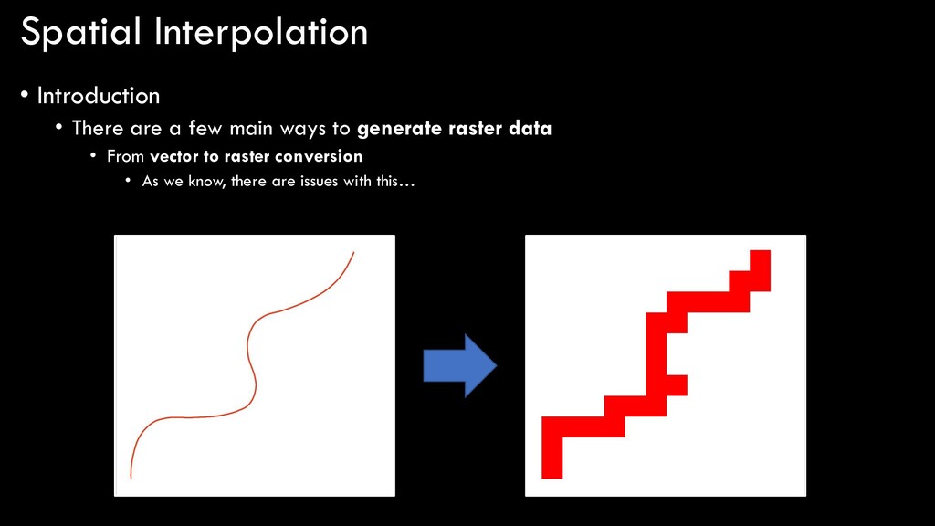
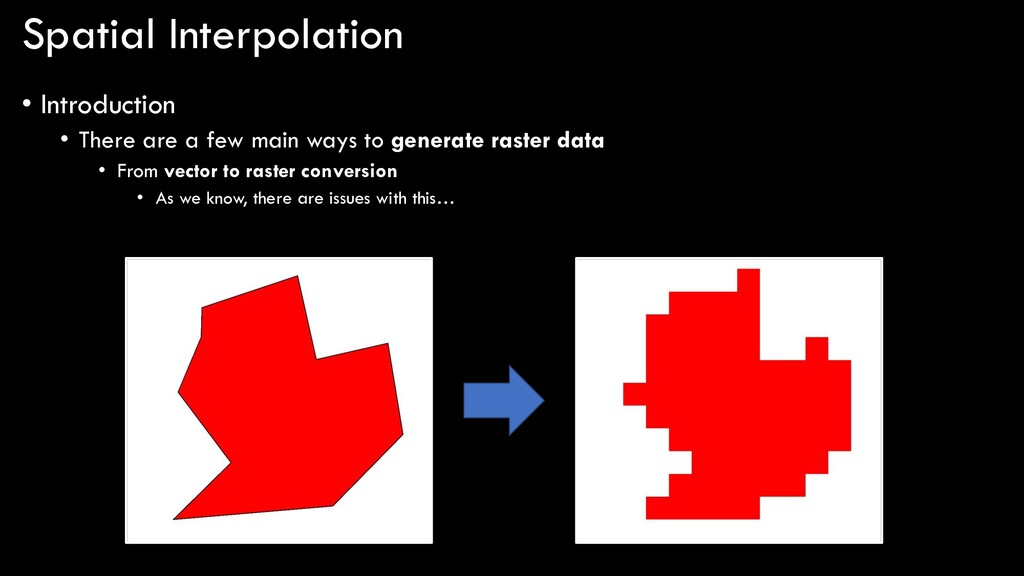
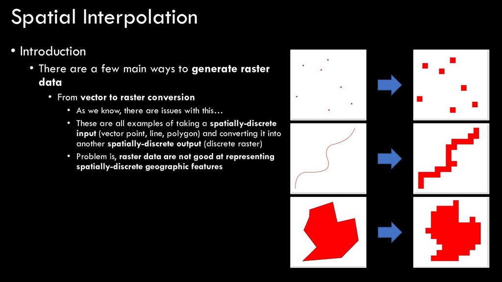
ways to generate raster data • From vector to raster conversion • As we know, there are issues with this… • These are all examples of taking a spatially-discrete input (vector point, line, polygon) and converting it into another spatially-discrete output (discrete raster) • Problem is, raster data are not good at representing spatially-discrete geographic features
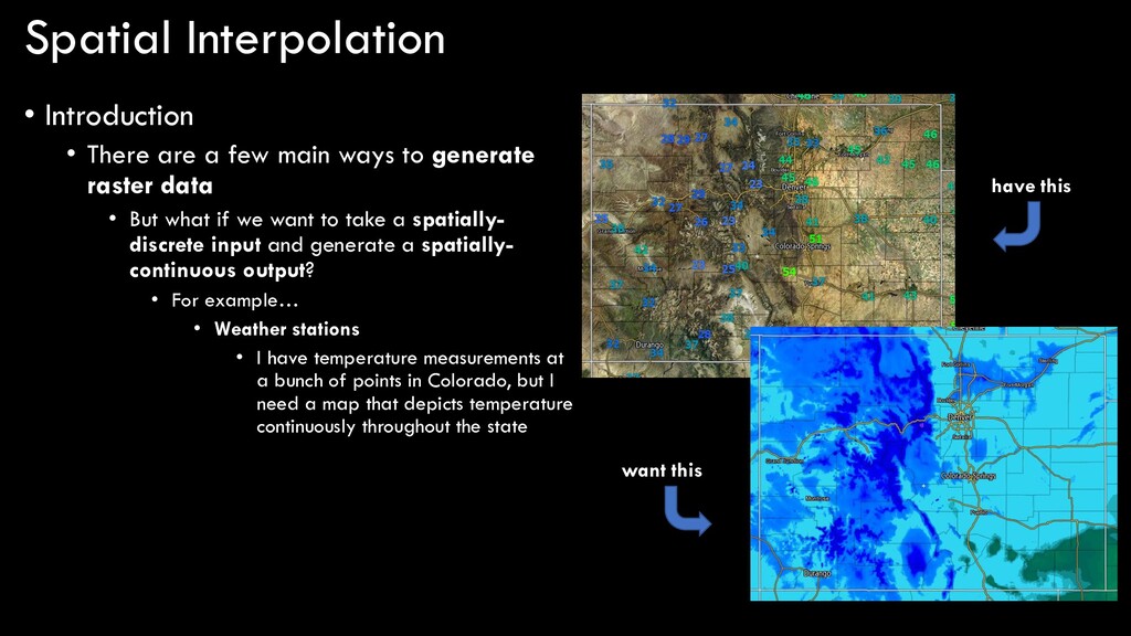
ways to generate raster data • But what if we want to take a spatially- discrete input and generate a spatially- continuous output? • For example… • Weather stations • I have temperature measurements at a bunch of points in Colorado, but I need a map that depicts temperature continuously throughout the state have this want this
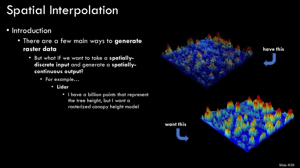
ways to generate raster data • But what if we want to take a spatially- discrete input and generate a spatially- continuous output? • For example… • Lidar • I have a billion points that represent the tree height, but I want a rasterized canopy height model Slide #20 have this want this
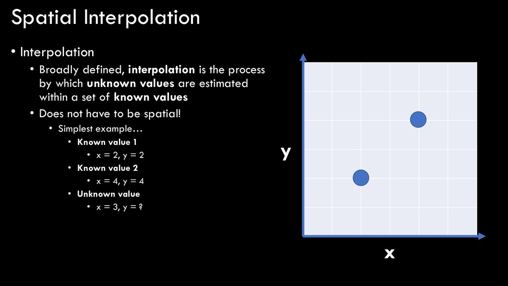
process by which unknown values are estimated within a set of known values • Does not have to be spatial! • Simplest example… • Known value 1 • x = 2, y = 2 • Known value 2 • x = 4, y = 4 • Unknown value • x = 3, y = ? x y
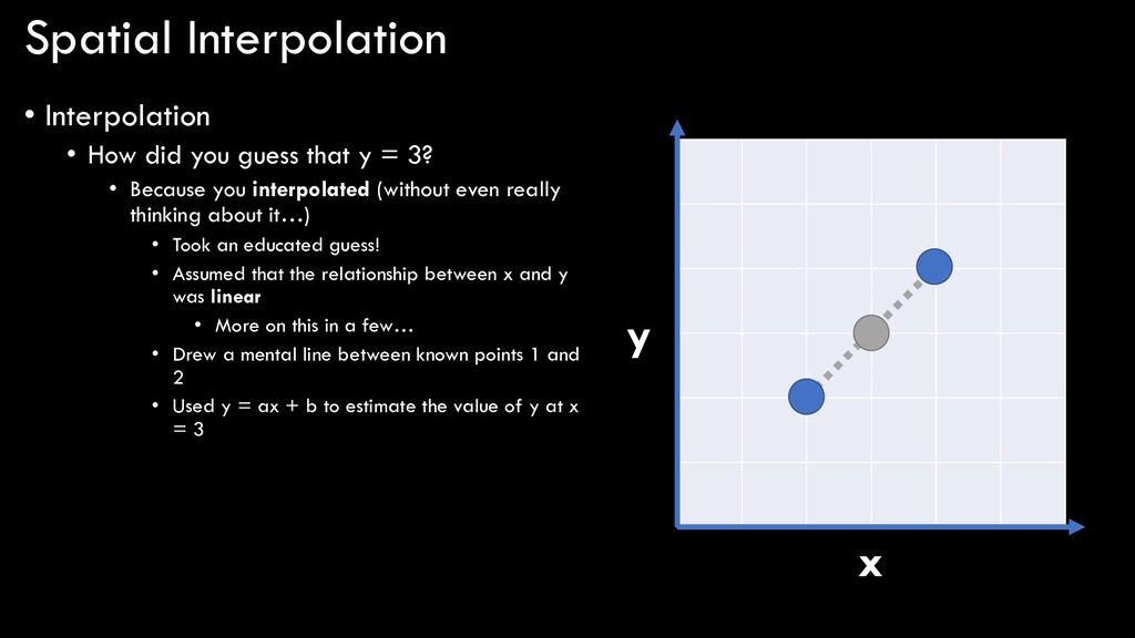
y = 3? • Because you interpolated (without even really thinking about it…) • Took an educated guess! • Assumed that the relationship between x and y was linear • More on this in a few… • Drew a mental line between known points 1 and 2 • Used y = ax + b to estimate the value of y at x = 3 x y
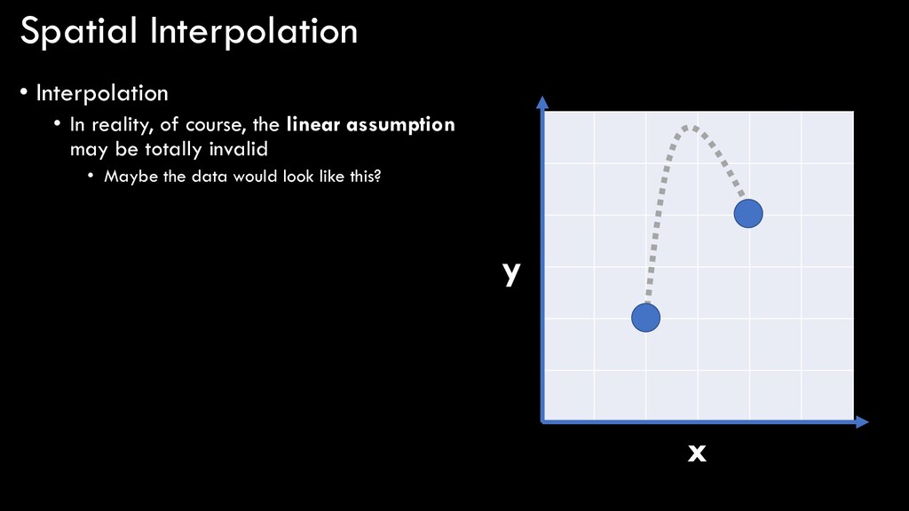
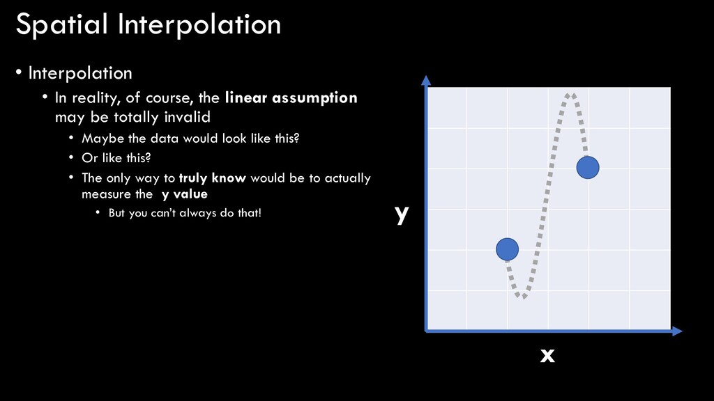
linear assumption may be totally invalid • Maybe the data would look like this? • Or like this? • The only way to truly know would be to actually measure the y value • But you can’t always do that! x y
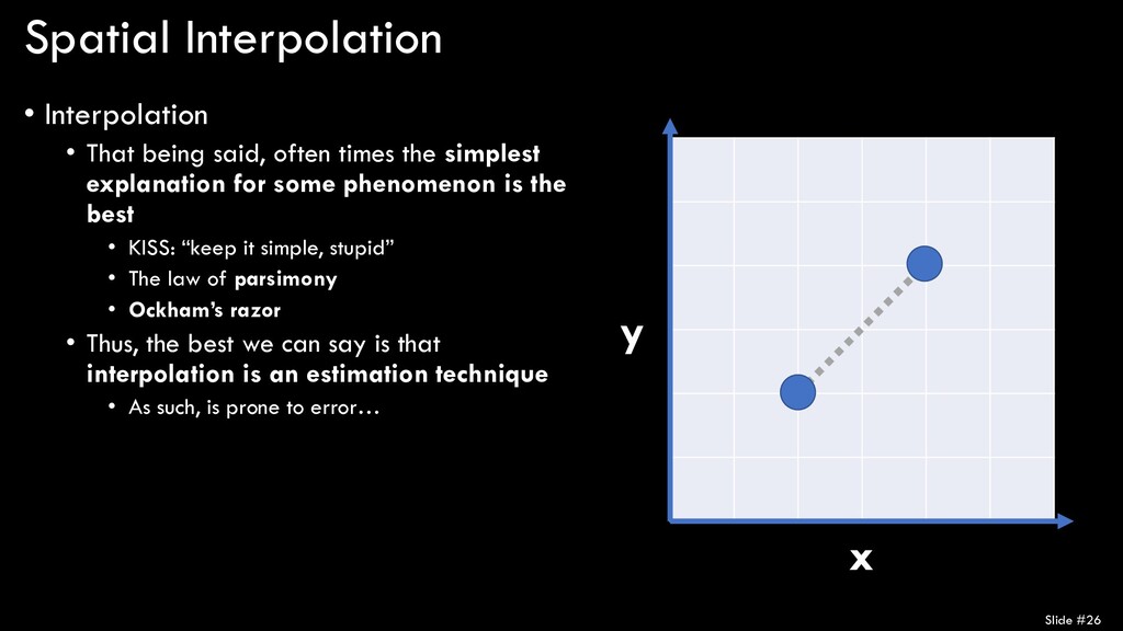
the simplest explanation for some phenomenon is the best • KISS: “keep it simple, stupid” • The law of parsimony • Ockham’s razor • Thus, the best we can say is that interpolation is an estimation technique • As such, is prone to error… Slide #26 x y
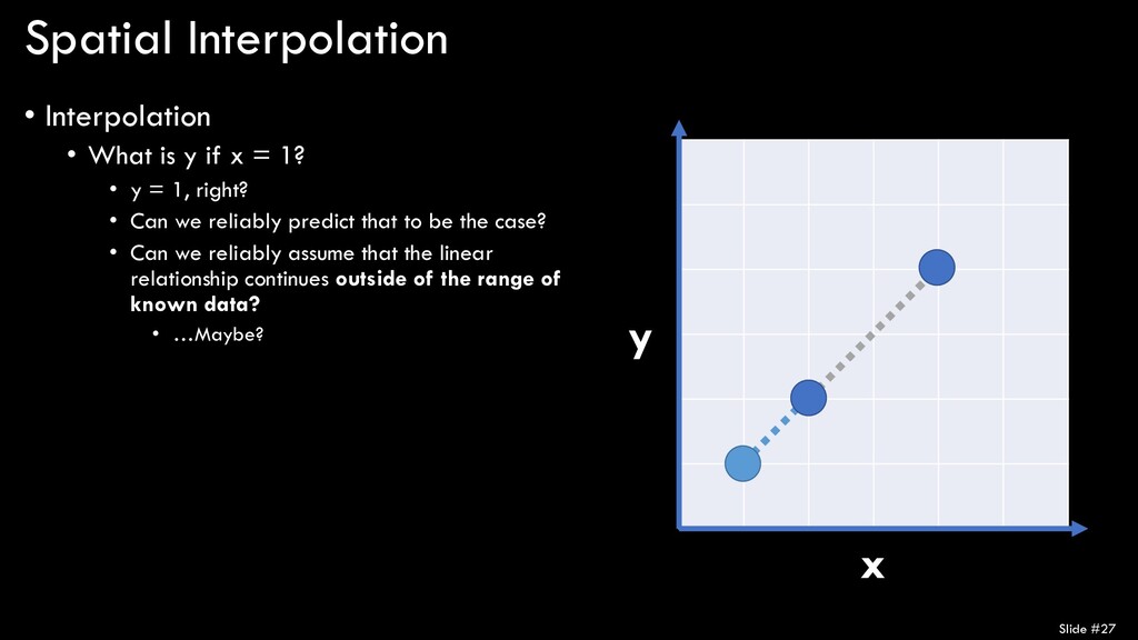
= 1? • y = 1, right? • Can we reliably predict that to be the case? • Can we reliably assume that the linear relationship continues outside of the range of known data? • …Maybe? Slide #27 x y
range of known values is known as extrapolation • Although they are both estimation techniques… • Interpolation is based on known values, and therefore is a valid approach • DO IT! (cautiously…) • Extrapolation is… A wild guess! • DON’T DO IT! Slide #28 x y
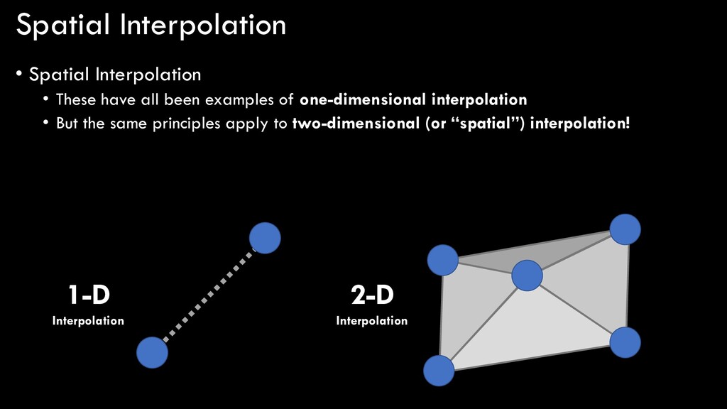
examples of one-dimensional interpolation • But the same principles apply to two-dimensional (or “spatial”) interpolation! 1-D Interpolation 2-D Interpolation
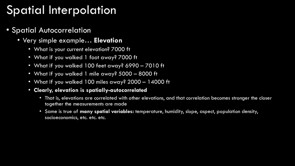
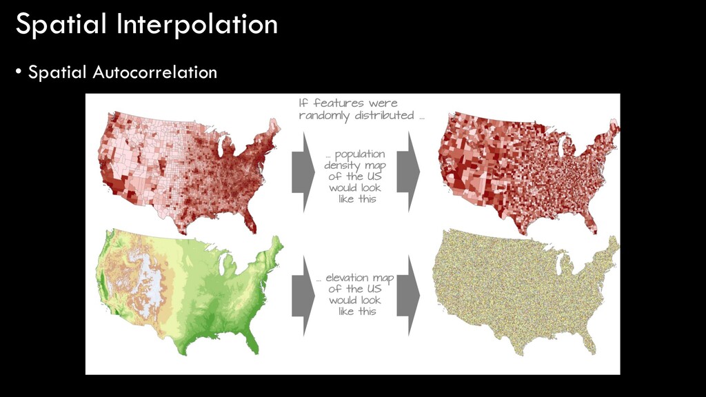
• What is your current elevation? 7000 ft • What if you walked 1 foot away? 7000 ft • What if you walked 100 feet away? 6990 – 7010 ft • What if you walked 1 mile away? 5000 – 8000 ft • What if you walked 100 miles away? 2000 – 14000 ft • Clearly, elevation is spatially-autocorrelated • That is, elevations are correlated with other elevations, and that correlation becomes stronger the closer together the measurements are made • Same is true of many spatial variables: temperature, humidity, slope, aspect, population density, socioeconomics, etc. etc. etc.
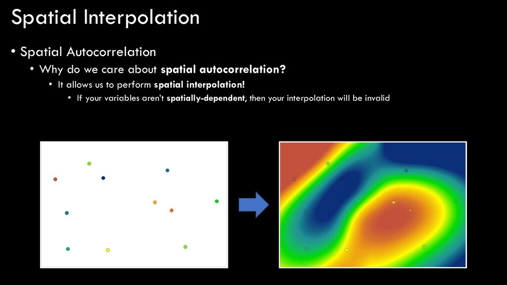
about spatial autocorrelation? • It allows us to perform spatial interpolation! • If your variables aren’t spatially-dependent, then your interpolation will be invalid
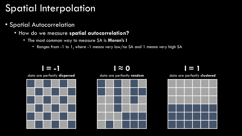
spatial autocorrelation? • The most common way to measure SA is Moran’s I • Ranges from -1 to 1, where -1 means very low/no SA and 1 means very high SA I = -1 data are perfectly dispersed I ≈ 0 data are perfectly random I = 1 data are perfectly clustered
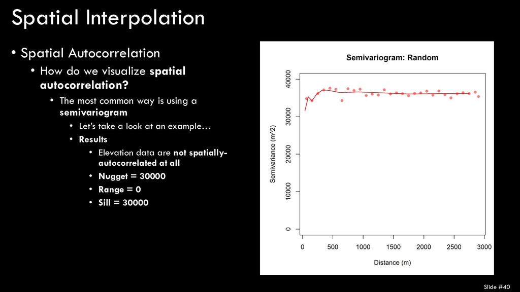
spatial autocorrelation? • The most common way is using a semivariogram • Displays the semivariance in a variable as a function of distance • What is semivariance? • Looks more complex than it really is… • A measure of how some value varies from itself based on distance • Take each point (xi ), subtract its z value (z(xi )) from every other point and calculate distance between (h), square the differences, sum them all up, and divide by 2 x the number of points (N)
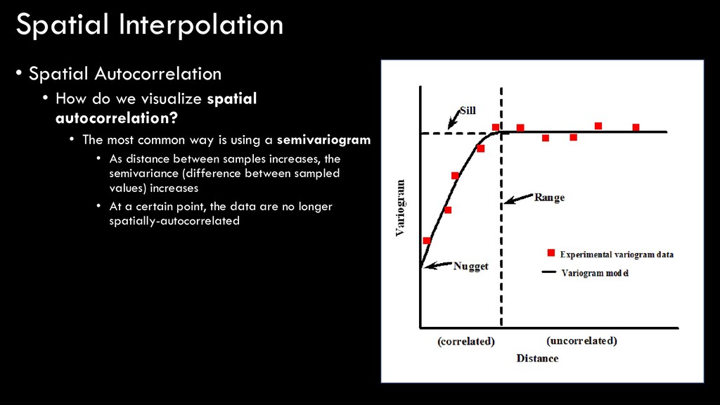
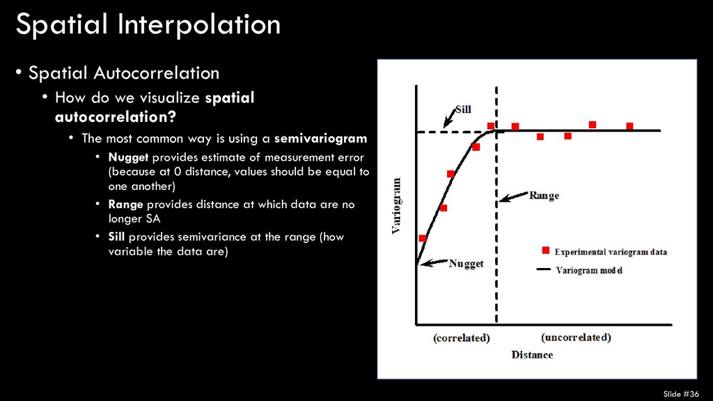
spatial autocorrelation? • The most common way is using a semivariogram • As distance between samples increases, the semivariance (difference between sampled values) increases • At a certain point, the data are no longer spatially-autocorrelated
spatial autocorrelation? • The most common way is using a semivariogram • Nugget provides estimate of measurement error (because at 0 distance, values should be equal to one another) • Range provides distance at which data are no longer SA • Sill provides semivariance at the range (how variable the data are) Slide #36
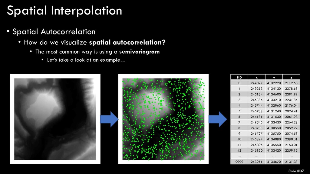
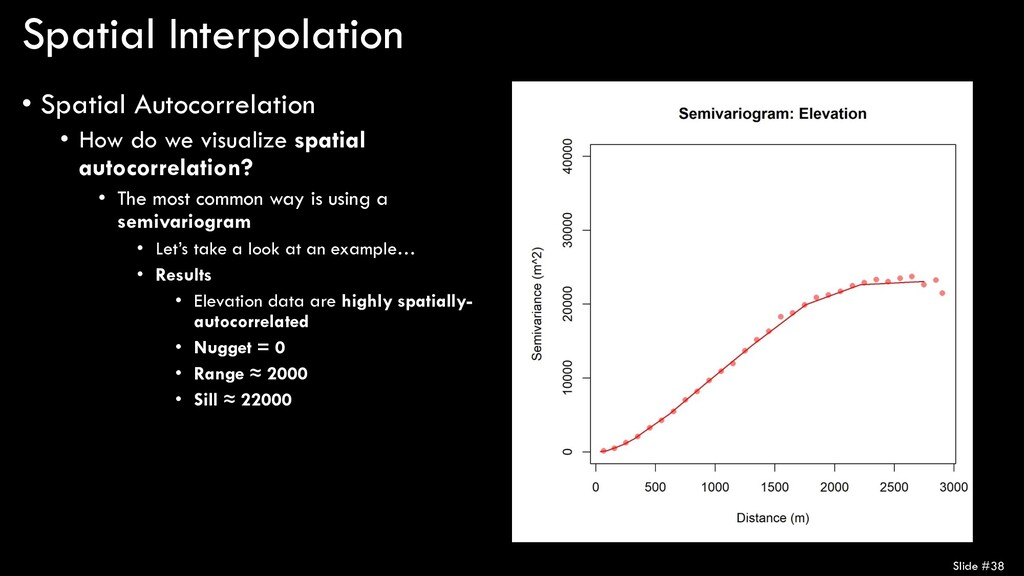
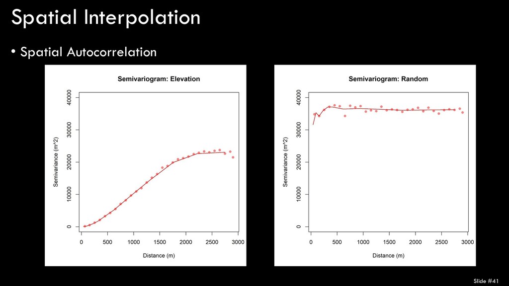
spatial autocorrelation? • The most common way is using a semivariogram • Let’s take a look at an example… • Results • Elevation data are highly spatially- autocorrelated • Nugget = 0 • Range ≈ 2000 • Sill ≈ 22000 Slide #38
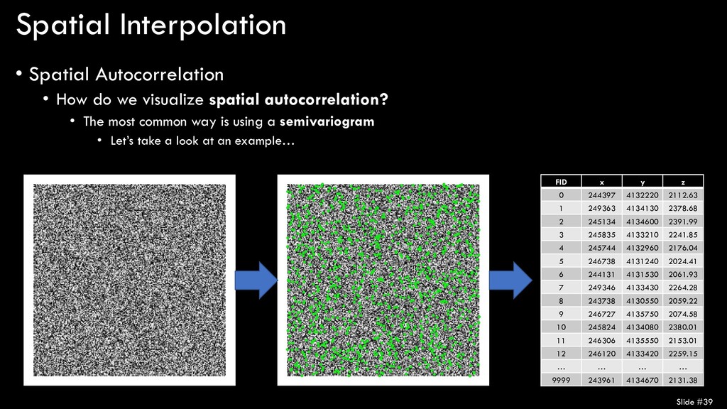
spatial autocorrelation? • The most common way is using a semivariogram • Let’s take a look at an example… • Results • Elevation data are not spatially- autocorrelated at all • Nugget = 30000 • Range = 0 • Sill = 30000 Slide #40
assume (or determine statistically) that our variable of interest is spatially-autocorrelated, then we can proceed with spatial interpolation • Again, most things in nature are spatially-autocorrelated, so interpolation is usually viable • However, the nature and strength of the autocorrelation can help dictate the type of interpolation to be performed
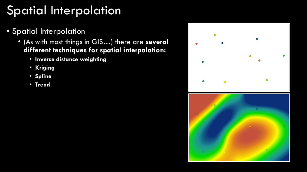
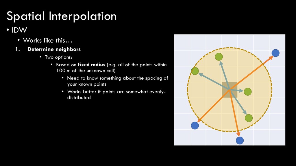
• Explicitly assumes Tobler’s 1st law • Everything is related to everything else, but near things are more related than distant things • Calculates unknown cell values based on values of nearby points with known values, weighting the influence of those points based on their proximity to the unknown cell
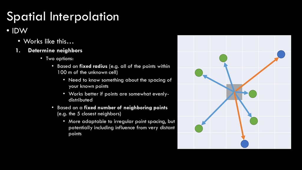
Two options: • Based on fixed radius (e.g. all of the points within 100 m of the unknown cell) • Need to know something about the spacing of your known points • Works better if points are somewhat evenly- distributed Spatial Interpolation
Two options: • Based on fixed radius (e.g. all of the points within 100 m of the unknown cell) • Need to know something about the spacing of your known points • Works better if points are somewhat evenly- distributed • Based on a fixed number of neighboring points (e.g. the 5 closest neighbors) • More adaptable to irregular point spacing, but potentially including influence from very distant points Spatial Interpolation
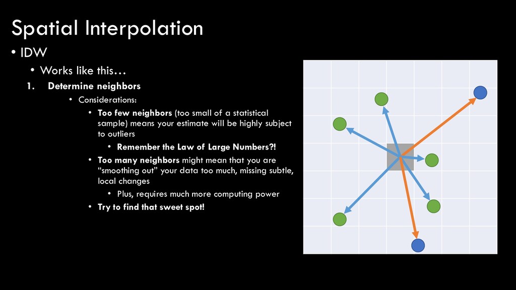
Considerations: • Too few neighbors (too small of a statistical sample) means your estimate will be highly subject to outliers • Remember the Law of Large Numbers?! • Too many neighbors might mean that you are “smoothing out” your data too much, missing subtle, local changes • Plus, requires much more computing power • Try to find that sweet spot! Spatial Interpolation
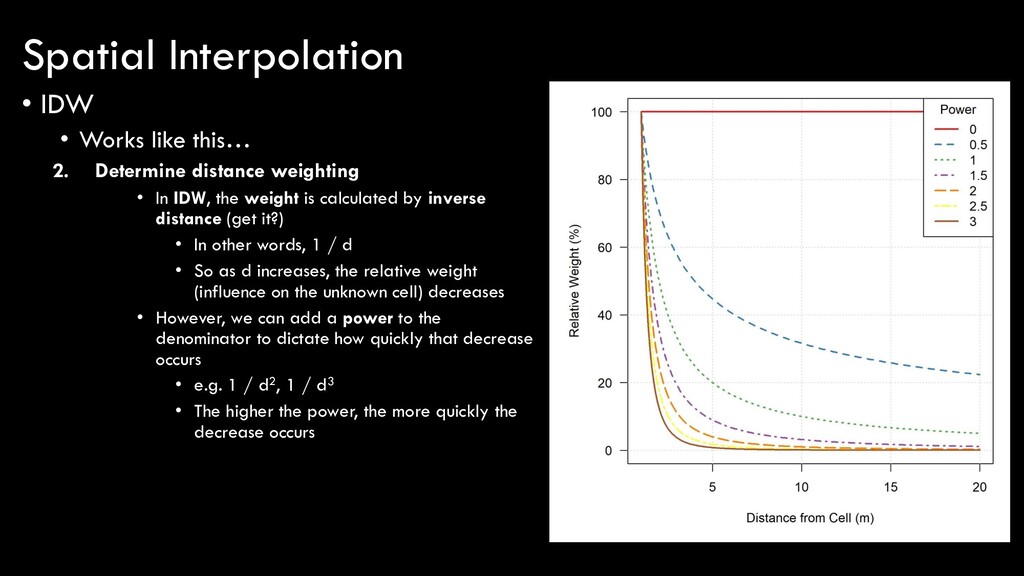
• In IDW, the weight is calculated by inverse distance (get it?) • In other words, 1 / d • So as d increases, the relative weight (influence on the unknown cell) decreases • However, we can add a power to the denominator to dictate how quickly that decrease occurs • e.g. 1 / d2, 1 / d3 • The higher the power, the more quickly the decrease occurs Spatial Interpolation
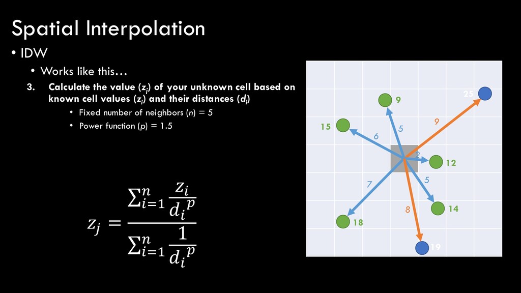
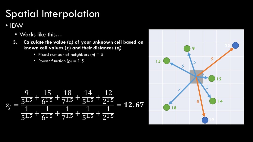
(zj ) of your unknown cell based on known cell values (zi ) and their distances (di ) • Fixed number of neighbors (n) = 5 • Power function (p) = 1.5 25 19 14 12 9 18 15 5 6 7 5 2 9 8 = σ=1 σ =1 1 Spatial Interpolation
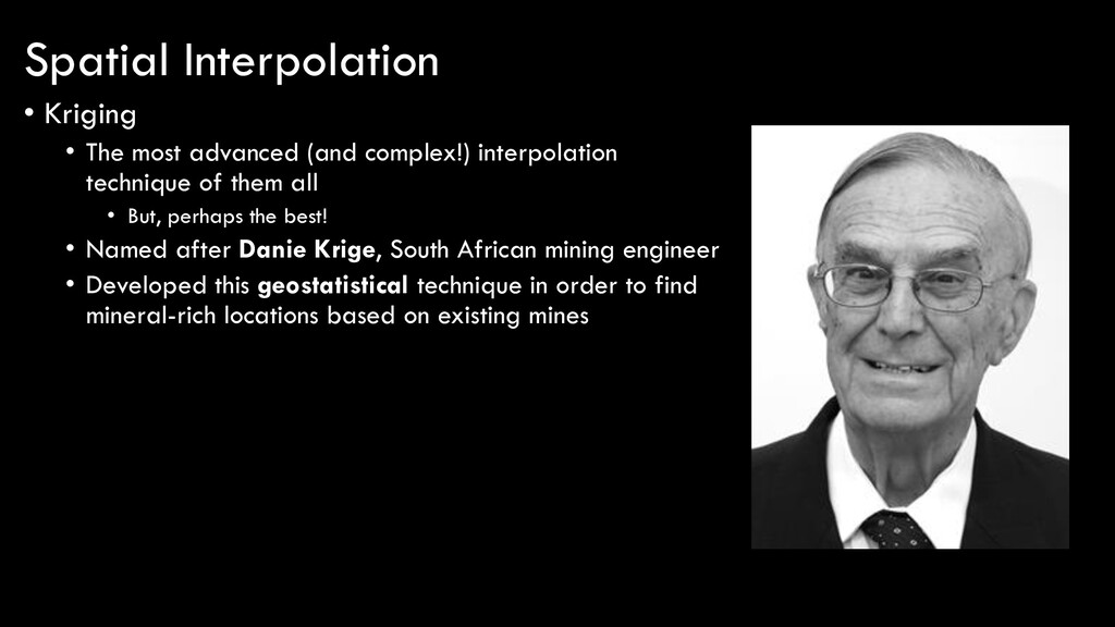
of them all • But, perhaps the best! • Named after Danie Krige, South African mining engineer • Developed this geostatistical technique in order to find mineral-rich locations based on existing mines Spatial Interpolation
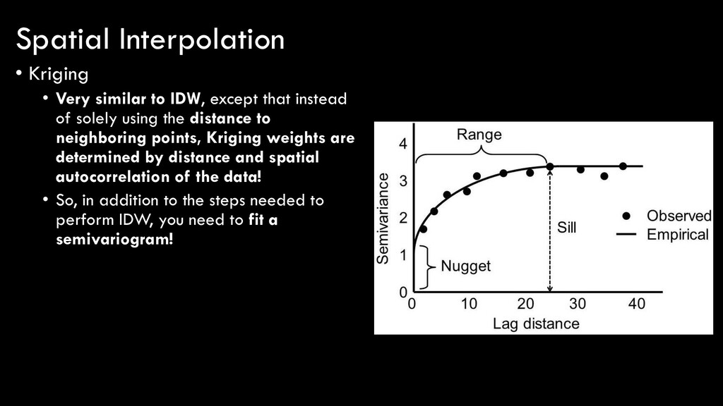
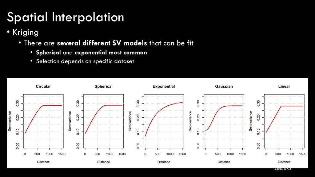
of solely using the distance to neighboring points, Kriging weights are determined by distance and spatial autocorrelation of the data! • So, in addition to the steps needed to perform IDW, you need to fit a semivariogram! Spatial Interpolation
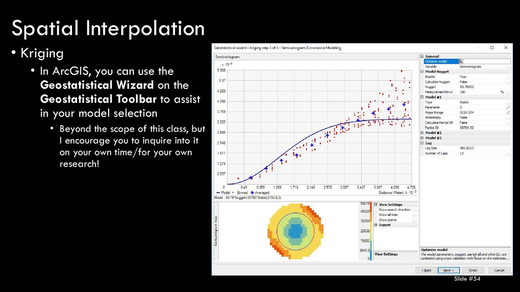
Wizard on the Geostatistical Toolbar to assist in your model selection • Beyond the scope of this class, but I encourage you to inquire into it on your own time/for your own research! Slide #54 Spatial Interpolation
“default” parameters, proper implementation requires an intimate knowledge of the geostatistics underlying the method as well as your data themselves • In some ways, the simpler algorithms (e.g. IDW, Spline) are more defensible, as they are relatively “naïve” methods and thus require a less-than-expert knowledge level Spatial Interpolation
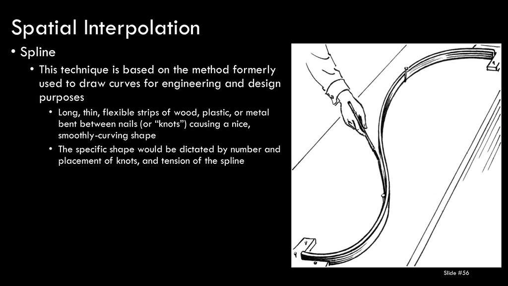
formerly used to draw curves for engineering and design purposes • Long, thin, flexible strips of wood, plastic, or metal bent between nails (or “knots”) causing a nice, smoothly-curving shape • The specific shape would be dictated by number and placement of knots, and tension of the spline Slide #56 Spatial Interpolation
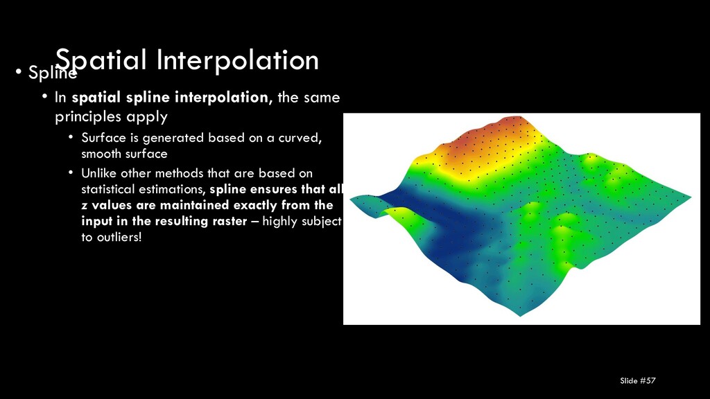
same principles apply • Surface is generated based on a curved, smooth surface • Unlike other methods that are based on statistical estimations, spline ensures that all z values are maintained exactly from the input in the resulting raster – highly subject to outliers! Slide #57
spline • Regularized produces a generally smoother surface • Tension produces a generally more rigid surface • Weight • For regularized, higher weights mean smoother output • For tension, higher weights mean rougher output • Number of points • For both, the number of nearest neighboring points used to create the localized spline Slide #58 Spatial Interpolation
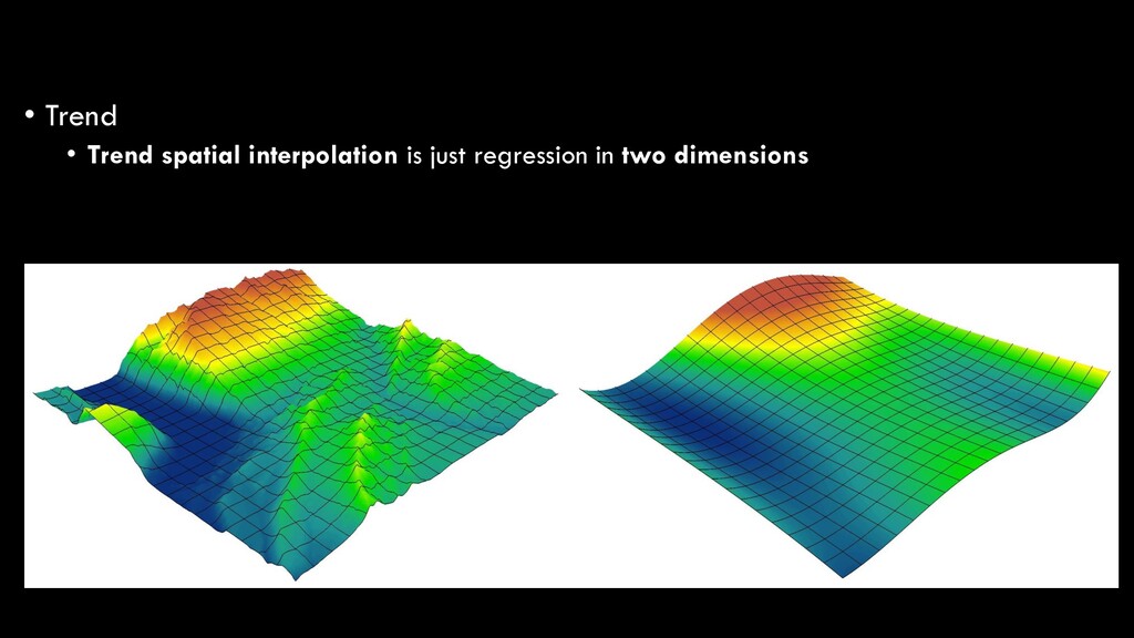
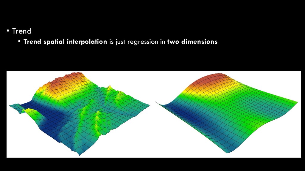
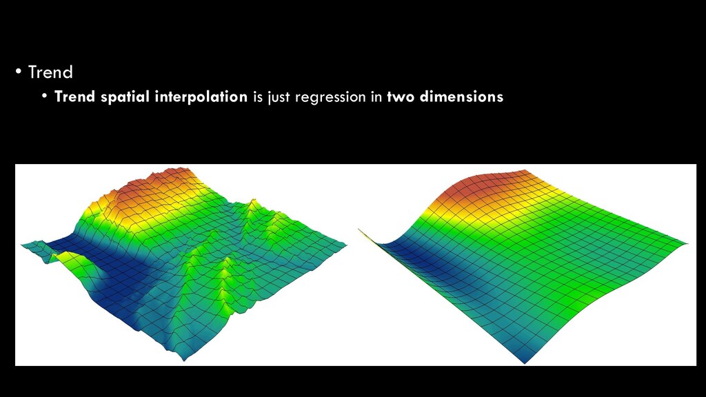
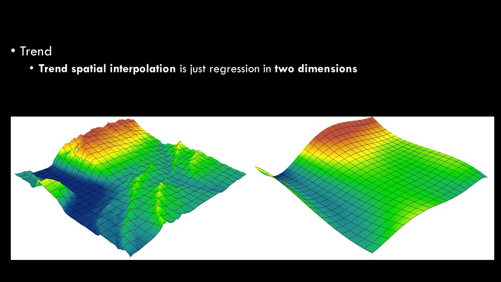
Regression analysis is the optimized fitting of a line or curve to derive a mathematical function that best fits the raw data • In our basic statistics lecture, we talked about the simplest form of regression: ordinary least squares (OLS) regression • Linear regression • y = ax + b • Predicting a dependent variable (y) based on an independent variable (x) Spatial Interpolation
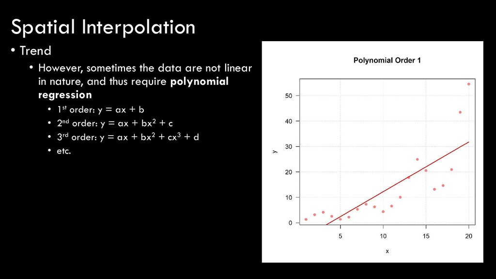
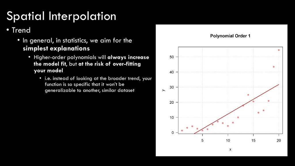
in nature, and thus require polynomial regression • 1st order: y = ax + b • 2nd order: y = ax + bx2 + c • 3rd order: y = ax + bx2 + cx3 + d • etc. Spatial Interpolation
the simplest explanations • Higher-order polynomials will always increase the model fit, but at the risk of over-fitting your model • i.e. instead of looking at the broader trend, your function is so specific that it won’t be generalizable to another, similar dataset Spatial Interpolation
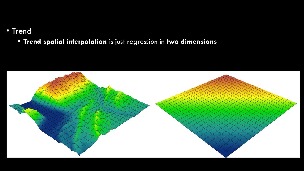
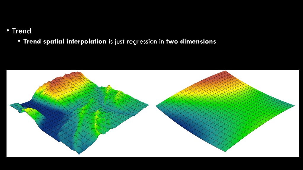
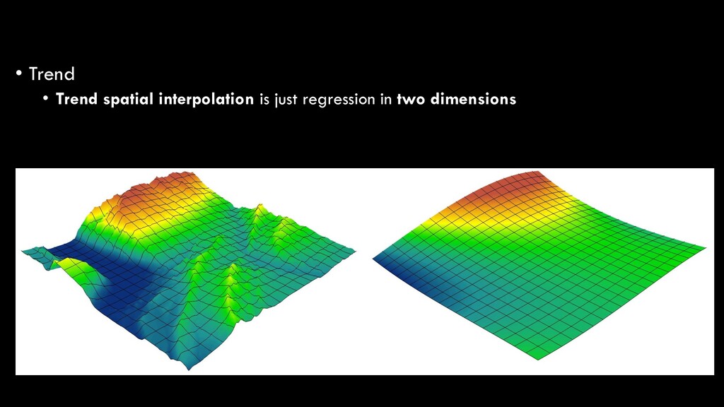
gradually over relatively broad areas • So, elevation is a bad example • But, atmospheric conditions (temperature, humidity, pollution, etc.) and aquatic conditions (temperature, pH, salinity) are good examples • Can also be used to “remove” broad-scale trends to reveal local phenomena • e.g. compare ambient (background) levels of O3 to local levels Spatial Interpolation