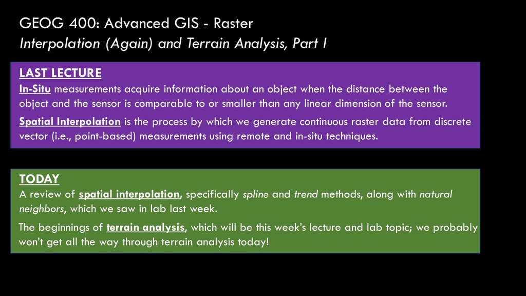
Analysis, Part I A review of spatial interpolation, specifically spline and trend methods, along with natural neighbors, which we saw in lab last week. LAST LECTURE TODAY In-Situ measurements acquire information about an object when the distance between the object and the sensor is comparable to or smaller than any linear dimension of the sensor. Spatial Interpolation is the process by which we generate continuous raster data from discrete vector (i.e., point-based) measurements using remote and in-situ techniques. The beginnings of terrain analysis, which will be this week’s lecture and lab topic; we probably won’t get all the way through terrain analysis today!
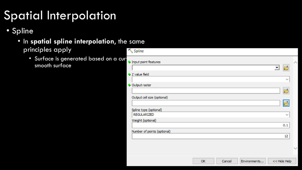
formerly used to draw curves for engineering and design purposes • Long, thin, flexible strips of wood, plastic, or metal bent between nails (or “knots”) causing a nice, smoothly-curving shape • The specific shape would be dictated by number and placement of knots, and tension of the spline Spatial Interpolation
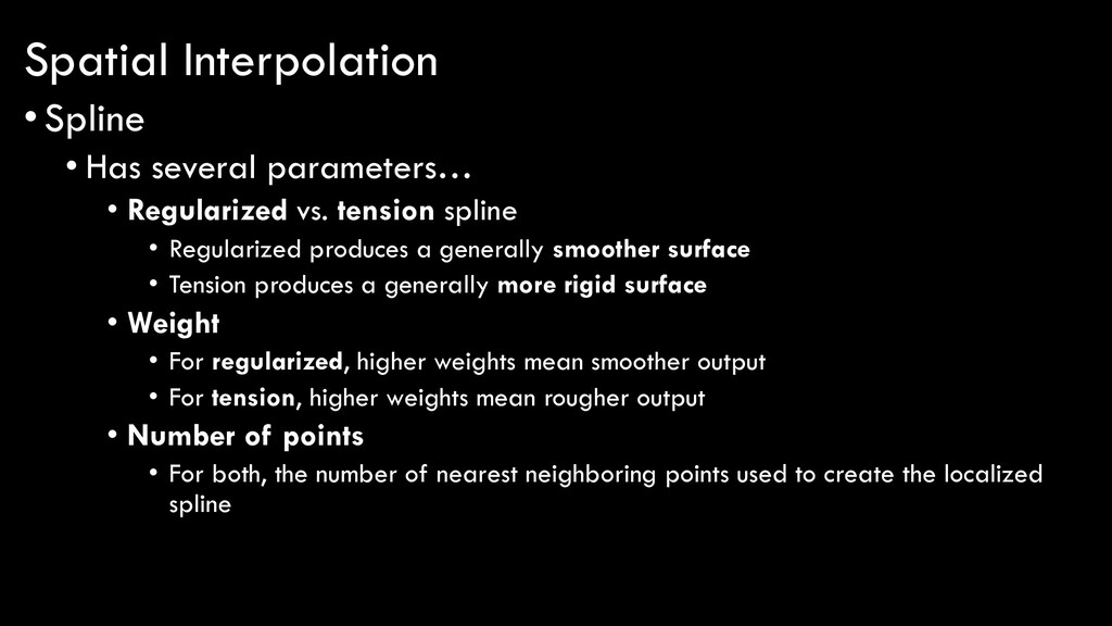
• Regularized produces a generally smoother surface • Tension produces a generally more rigid surface • Weight • For regularized, higher weights mean smoother output • For tension, higher weights mean rougher output • Number of points • For both, the number of nearest neighboring points used to create the localized spline Spatial Interpolation
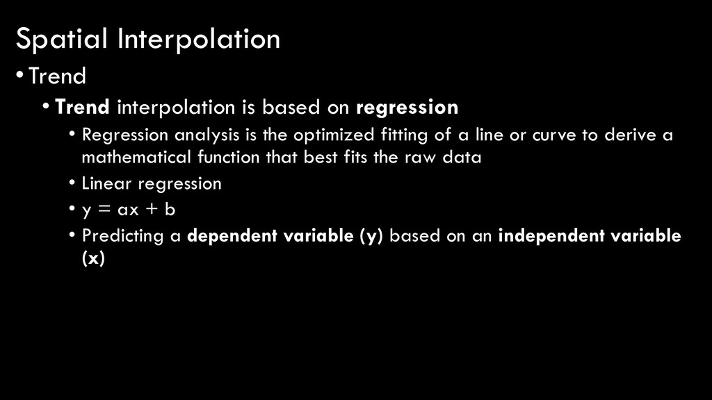
analysis is the optimized fitting of a line or curve to derive a mathematical function that best fits the raw data • Linear regression • y = ax + b • Predicting a dependent variable (y) based on an independent variable (x) Spatial Interpolation
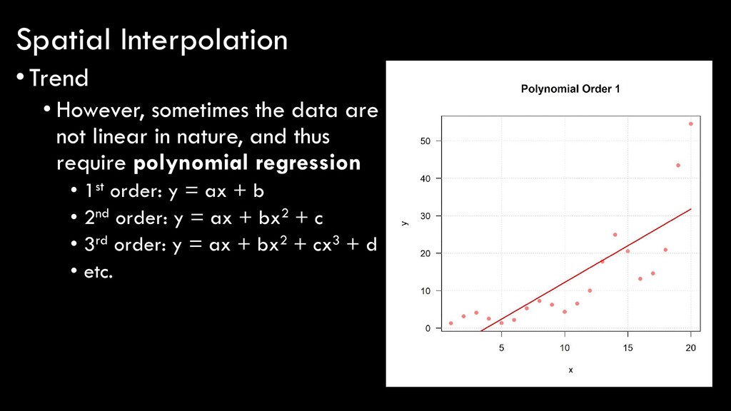
nature, and thus require polynomial regression • 1st order: y = ax + b • 2nd order: y = ax + bx2 + c • 3rd order: y = ax + bx2 + cx3 + d • etc. Spatial Interpolation
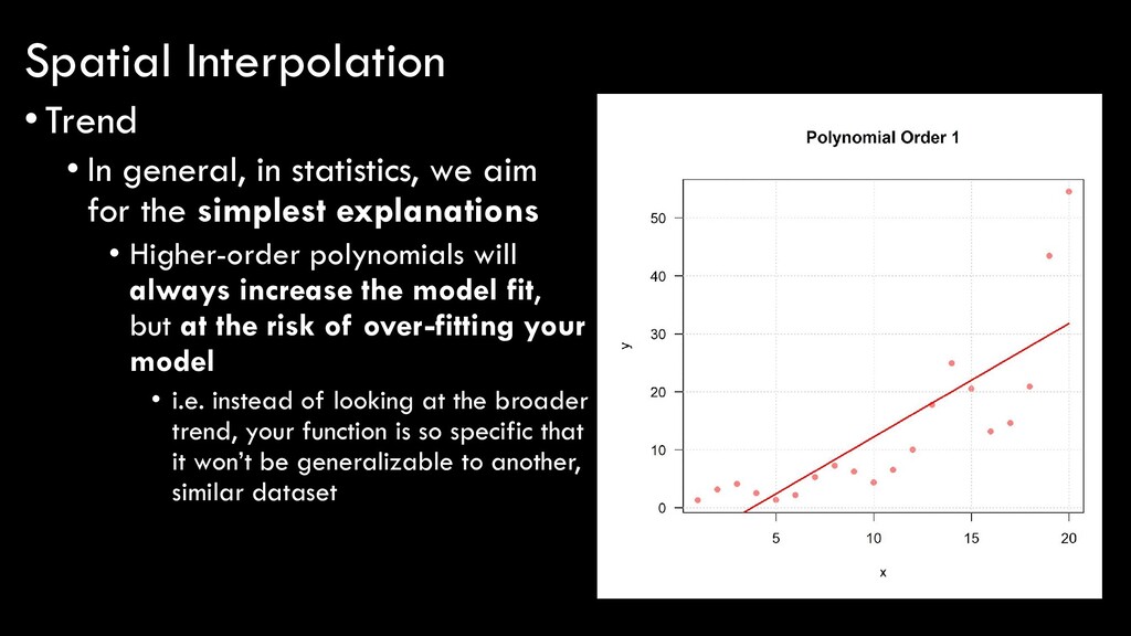
simplest explanations • Higher-order polynomials will always increase the model fit, but at the risk of over-fitting your model • i.e. instead of looking at the broader trend, your function is so specific that it won’t be generalizable to another, similar dataset Spatial Interpolation
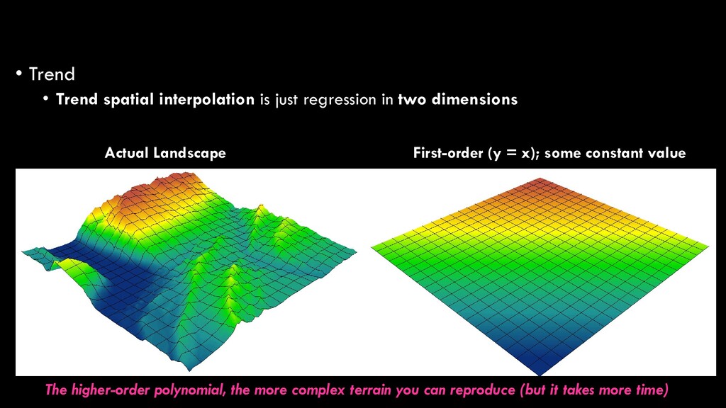
two dimensions raw data 1st order polynomial trend surface First-order (y = x); some constant value Actual Landscape The higher-order polynomial, the more complex terrain you can reproduce (but it takes more time)
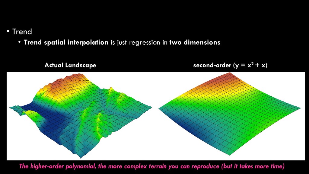
two dimensions raw data 2nd order polynomial trend surface second-order (y = x2 + x) Actual Landscape The higher-order polynomial, the more complex terrain you can reproduce (but it takes more time)
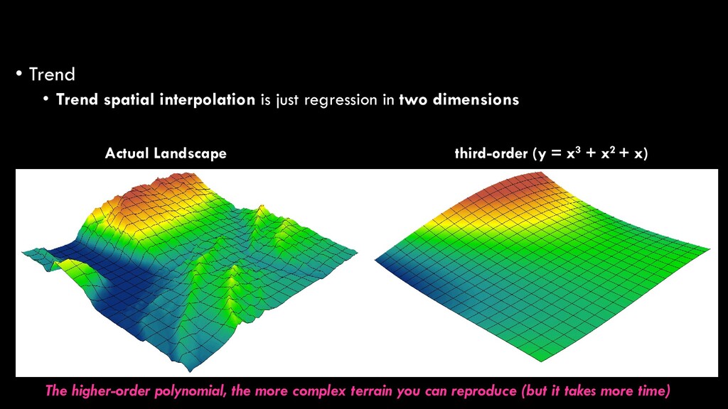
two dimensions raw data 3rd order polynomial trend surface third-order (y = x3 + x2 + x) Actual Landscape The higher-order polynomial, the more complex terrain you can reproduce (but it takes more time)
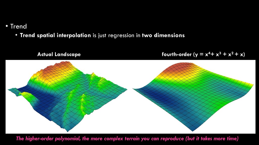
two dimensions raw data 4th order polynomial trend surface fourth-order (y = x4+ x3 + x2 + x) Actual Landscape The higher-order polynomial, the more complex terrain you can reproduce (but it takes more time)
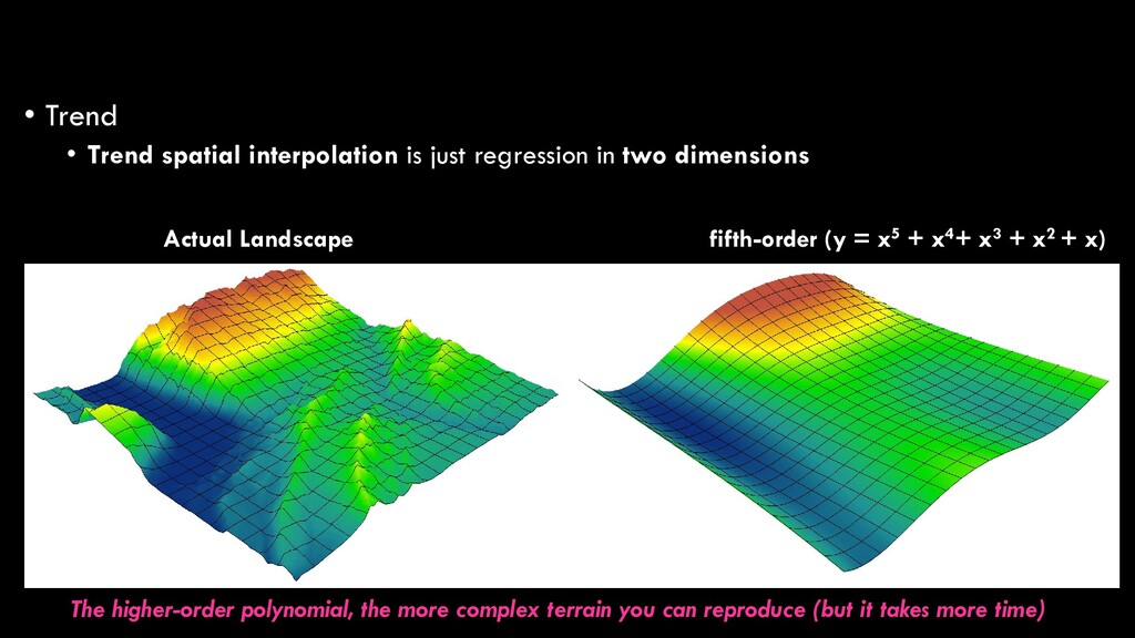
two dimensions raw data 5th order polynomial trend surface fifth-order (y = x5 + x4+ x3 + x2 + x) Actual Landscape The higher-order polynomial, the more complex terrain you can reproduce (but it takes more time)
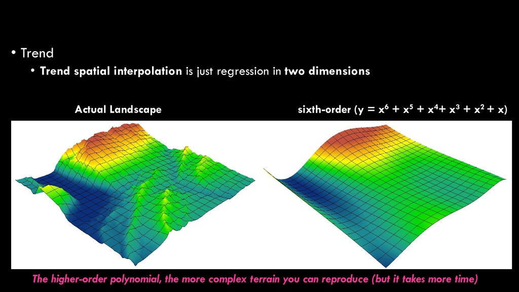
two dimensions raw data 6th order polynomial trend surface sixth-order (y = x6 + x5 + x4+ x3 + x2 + x) Actual Landscape The higher-order polynomial, the more complex terrain you can reproduce (but it takes more time)
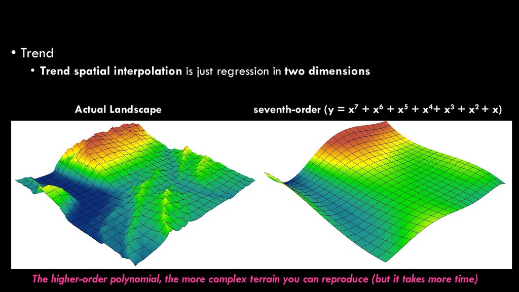
two dimensions raw data 7th order polynomial trend surface seventh-order (y = x7 + x6 + x5 + x4+ x3 + x2 + x) Actual Landscape The higher-order polynomial, the more complex terrain you can reproduce (but it takes more time)
over relatively broad areas • So, elevation is a bad example • But, atmospheric conditions (temperature, humidity, pollution, etc.) and aquatic conditions (temperature, pH, salinity) are good examples • Can also be used to “remove” broad-scale trends to reveal local phenomena • e.g. compare ambient (background) levels of O3 to local levels Spatial Interpolation
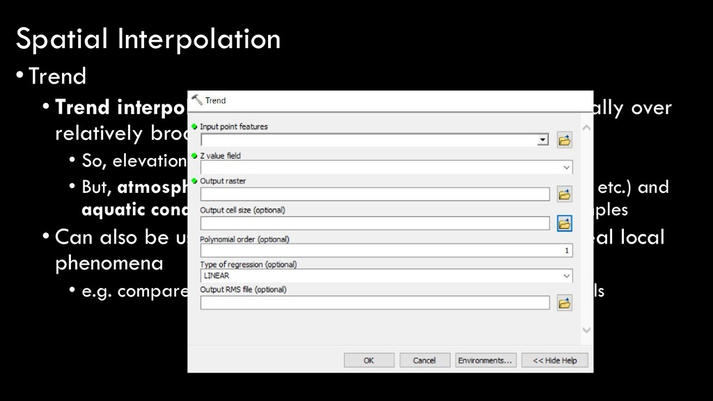
over relatively broad areas • So, elevation is a bad example • But, atmospheric conditions (temperature, humidity, pollution, etc.) and aquatic conditions (temperature, pH, salinity) are good examples • Can also be used to “remove” broad-scale trends to reveal local phenomena • e.g. compare ambient (background) levels of O3 to local levels Spatial Interpolation
about digital elevation models (DEMs) • What they are • Who creates and maintains them • How they’re created • Where they’re currently available • The focus of today’s lecture is the next, logical question: • What can we do with them?! • Terrain modeling applications in ArcGIS Deriving additional descriptors of land shape (i.e., morphometry) from elevation/terrain data.
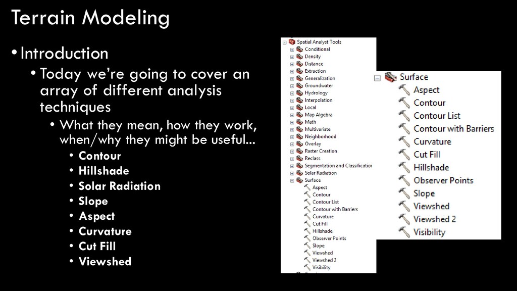
array of different analysis techniques • What they mean, how they work, when/why they might be useful... • Contour • Hillshade • Solar Radiation • Slope • Aspect • Curvature • Cut Fill • Viewshed
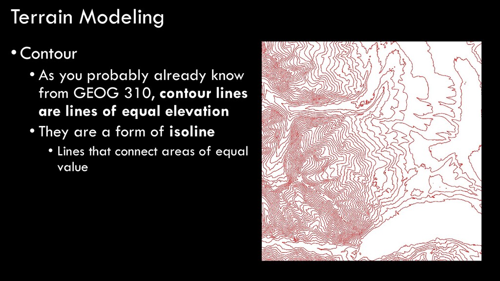
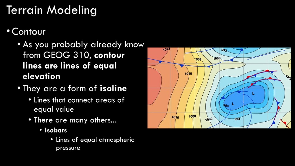
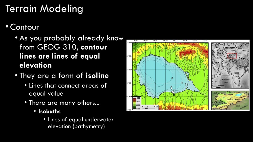
GEOG 310, contour lines are lines of equal elevation • They are a form of isoline • Lines that connect areas of equal value • There are many others... • Isobars • Lines of equal atmospheric pressure
GEOG 310, contour lines are lines of equal elevation • They are a form of isoline • Lines that connect areas of equal value • There are many others... • Isotherm • Lines of equal temperature
GEOG 310, contour lines are lines of equal elevation • They are a form of isoline • Lines that connect areas of equal value • There are many others... • Isobaths • Lines of equal underwater elevation (bathymetry)
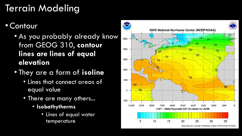
GEOG 310, contour lines are lines of equal elevation • They are a form of isoline • Lines that connect areas of equal value • There are many others... • Isobathytherms • Lines of equal water temperature
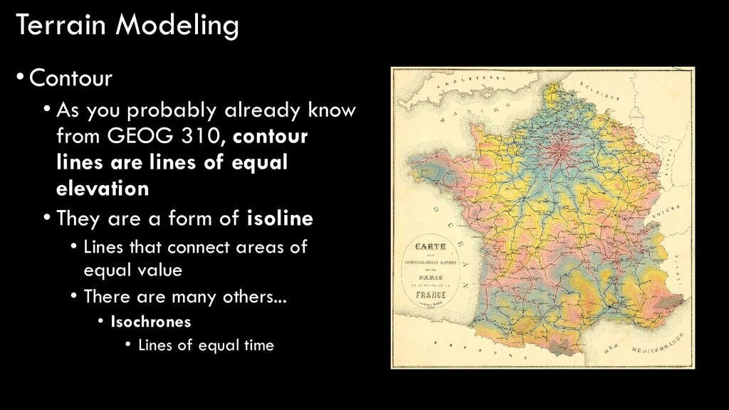
GEOG 310, contour lines are lines of equal elevation • They are a form of isoline • Lines that connect areas of equal value • There are many others... • Isochrones • Lines of equal time
GEOG 310, contour lines are lines of equal elevation • They are a form of isoline • Lines that connect areas of equal value • There are many others... • Isotachs • Lines of equal wind speed
GEOG 310, contour lines are lines of equal elevation • They are a form of isoline • Lines that connect areas of equal value • There are many others... • Isohyets • Lines of equal precipitation
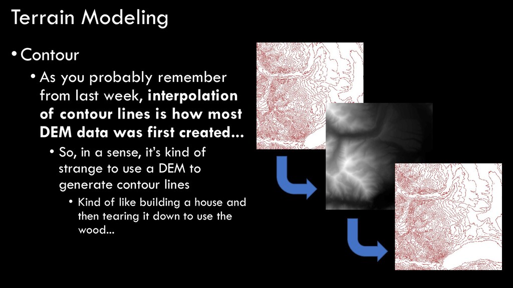
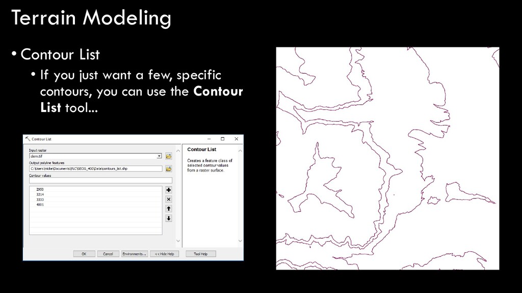
week, interpolation of contour lines is how most DEM data was first created... • So, in a sense, it’s kind of strange to use a DEM to generate contour lines • Kind of like building a house and then tearing it down to use the wood...
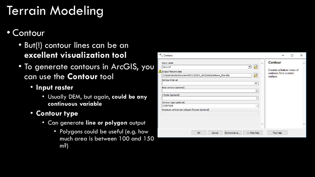
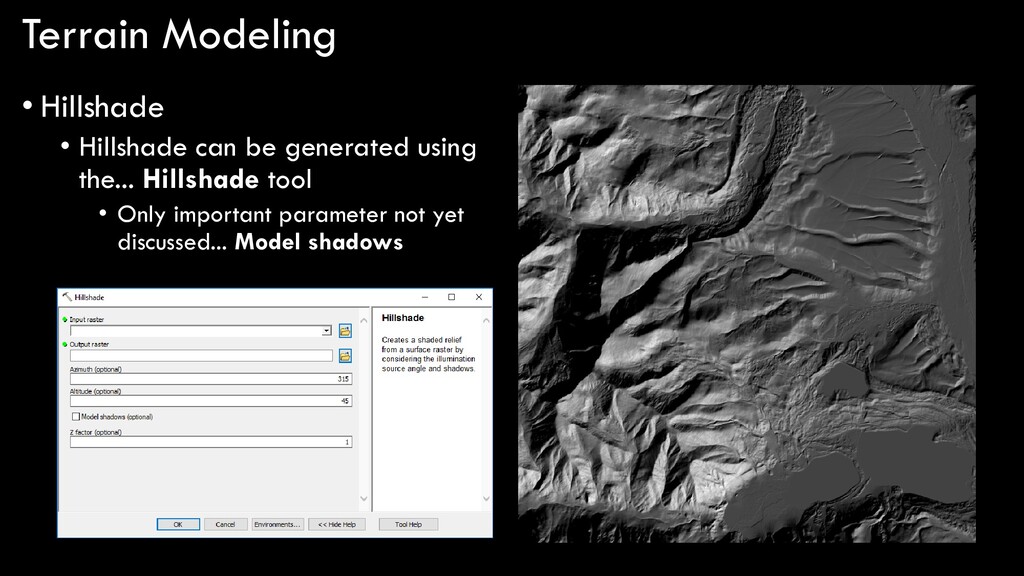
an excellent visualization tool • To generate contours in ArcGIS, you can use the Contour tool • Input raster • Usually DEM, but again, could be any continuous variable • Contour type • Can generate line or polygon output • Polygons could be useful (e.g. how much area is between 100 and 150 m?)
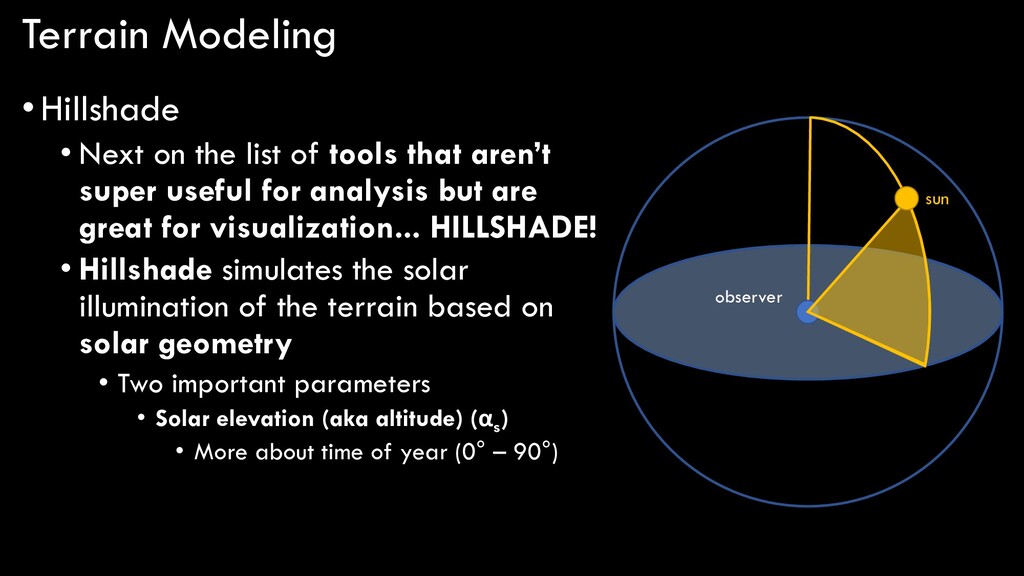
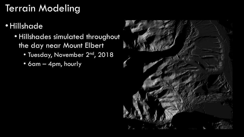
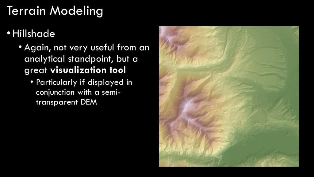
that aren’t super useful for analysis but are great for visualization... HILLSHADE! • Hillshade simulates the solar illumination of the terrain based on solar geometry • Two important parameters • Solar elevation (aka altitude) (αs ) • More about time of year (0° – 90°) observer sun
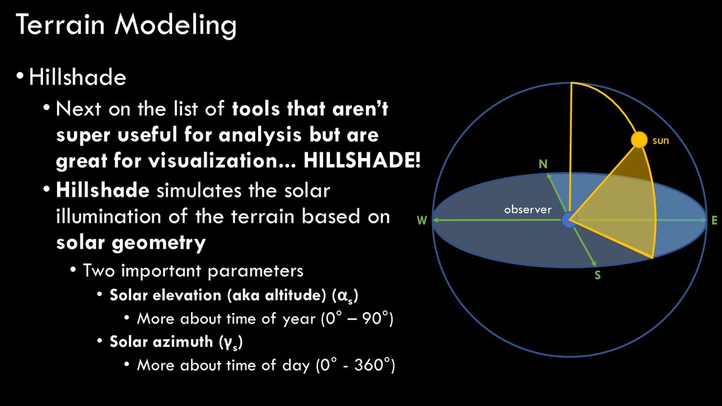
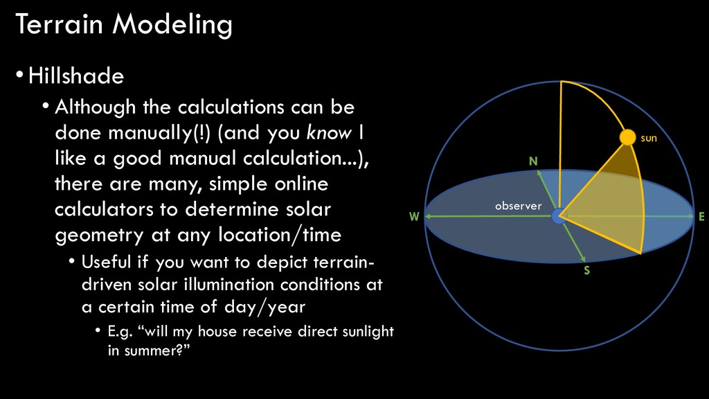
that aren’t super useful for analysis but are great for visualization... HILLSHADE! • Hillshade simulates the solar illumination of the terrain based on solar geometry • Two important parameters • Solar elevation (aka altitude) (αs ) • More about time of year (0° – 90°) • Solar azimuth (γs ) • More about time of day (0° - 360°) observer sun N W S E
manually(!) (and you know I like a good manual calculation...), there are many, simple online calculators to determine solar geometry at any location/time • Useful if you want to depict terrain- driven solar illumination conditions at a certain time of day/year • E.g. “will my house receive direct sunlight in summer?” observer sun N W S E
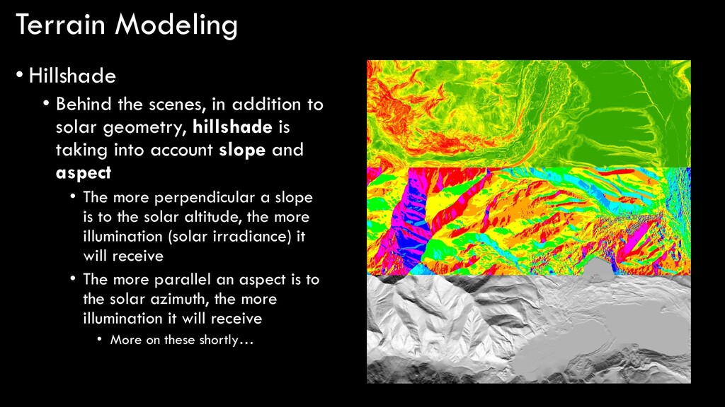
to solar geometry, hillshade is taking into account slope and aspect • The more perpendicular a slope is to the solar altitude, the more illumination (solar irradiance) it will receive • The more parallel an aspect is to the solar azimuth, the more illumination it will receive • More on these shortly…
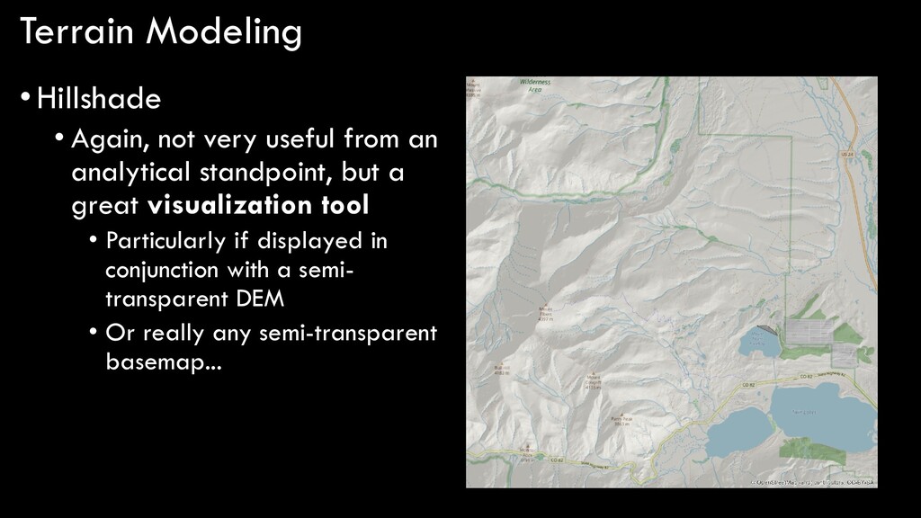
analytical standpoint, but a great visualization tool • Particularly if displayed in conjunction with a semi- transparent DEM • Or really any semi-transparent basemap...
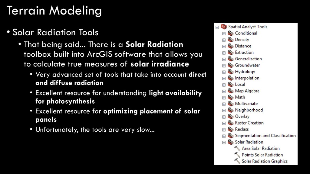
There is a Solar Radiation toolbox built into ArcGIS software that allows you to calculate true measures of solar irradiance • Very advanced set of tools that take into account direct and diffuse radiation • Excellent resource for understanding light availability for photosynthesis • Excellent resource for optimizing placement of solar panels • Unfortunately, the tools are very slow...
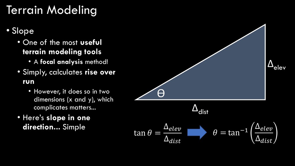
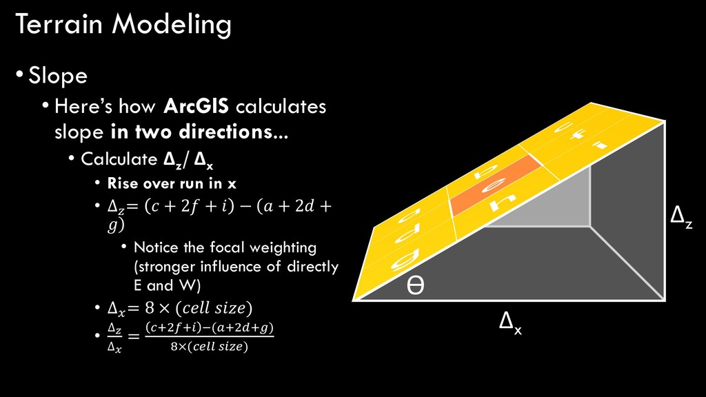
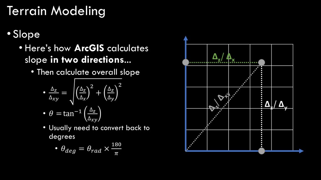
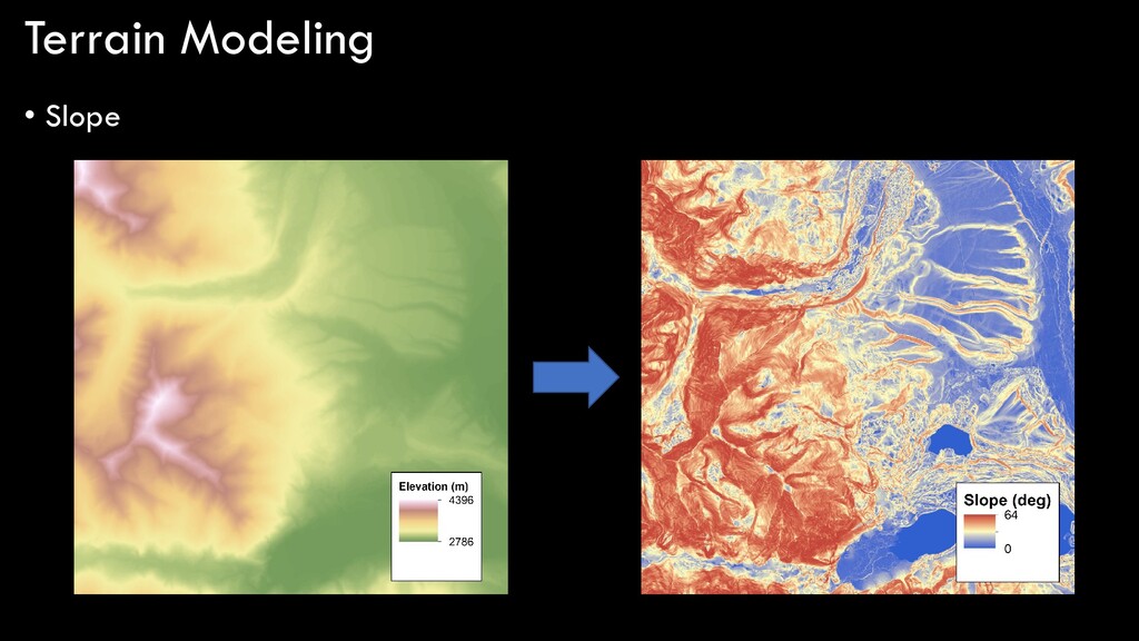
terrain modeling tools • A focal analysis method! • Simply, calculates rise over run • However, it does so in two dimensions (x and y), which complicates matters... • Here’s slope in one direction... Simple ϴ Δelev Δdist tan = ∆ ∆ = tan−1 ∆ ∆
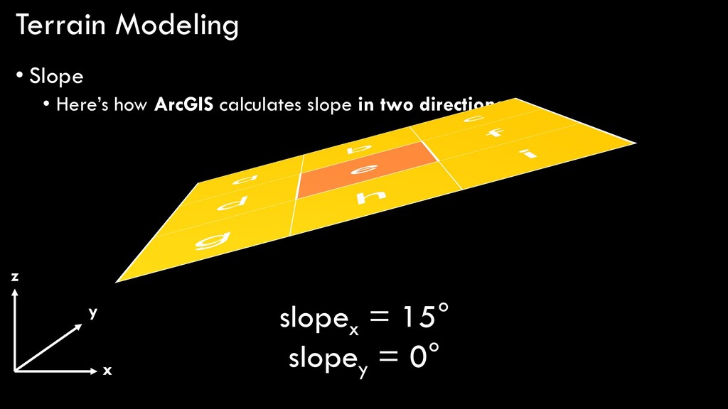
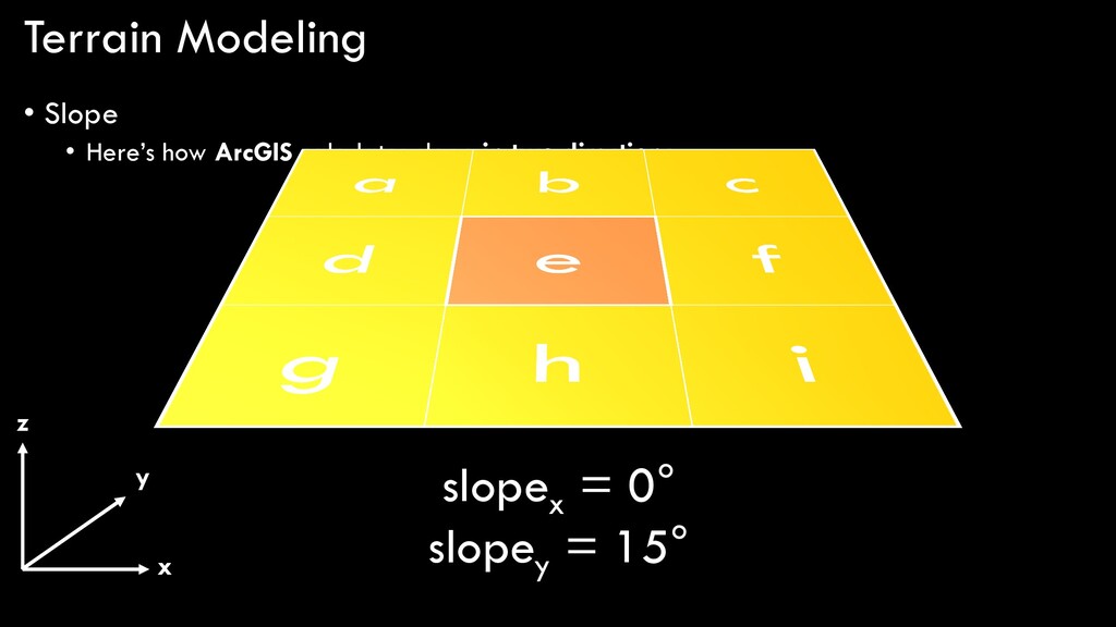
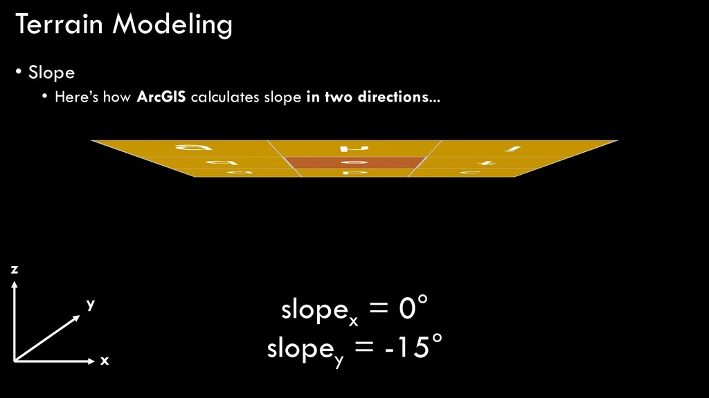
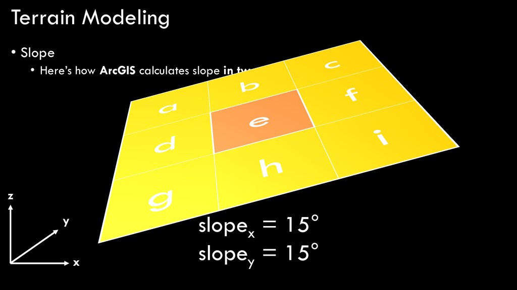
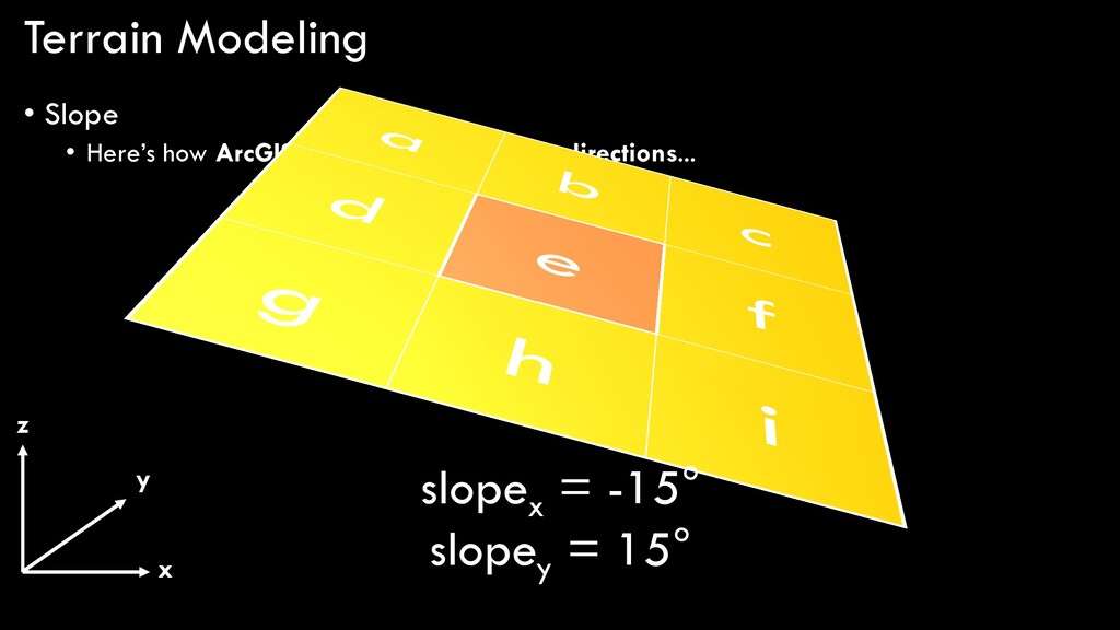
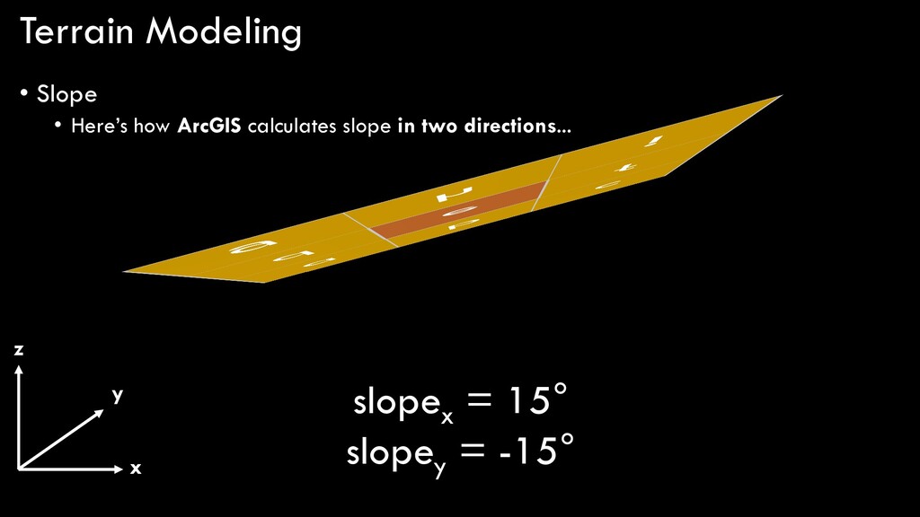
in two directions... • Uses a 3x3 focal neighborhood to calculate slope of the target cell NW N NE W E SW S SE reference analysis window 3 x 3 neighborhood target analysis cell
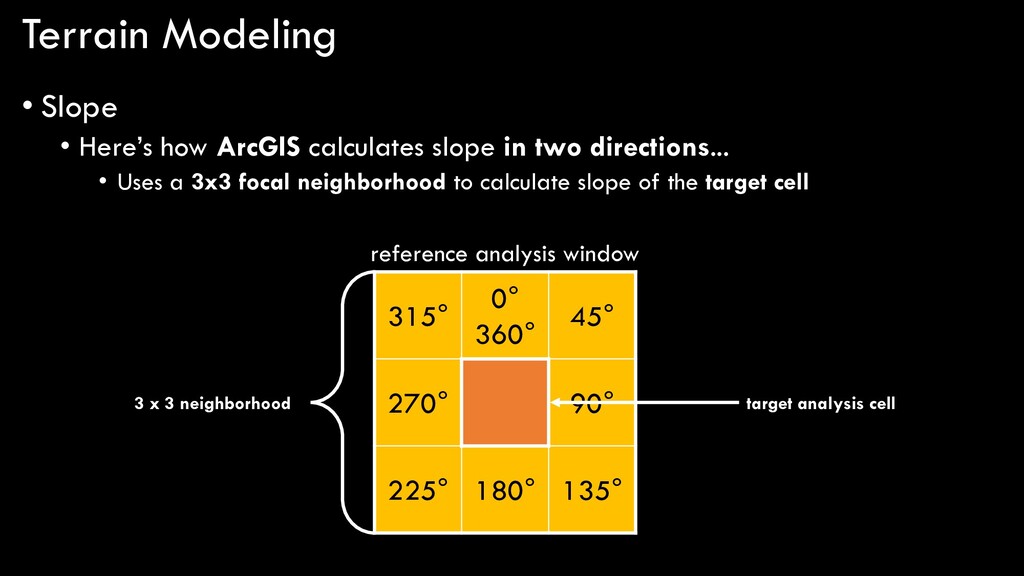
in two directions... • Uses a 3x3 focal neighborhood to calculate slope of the target cell 315° 0° 360° 45° 270° 90° 225° 180° 135° reference analysis window 3 x 3 neighborhood target analysis cell
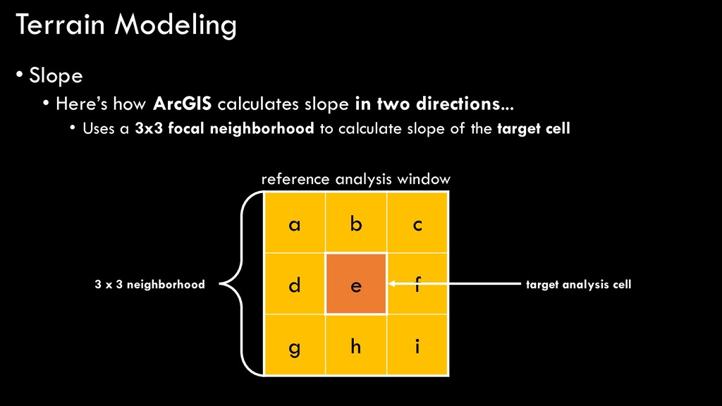
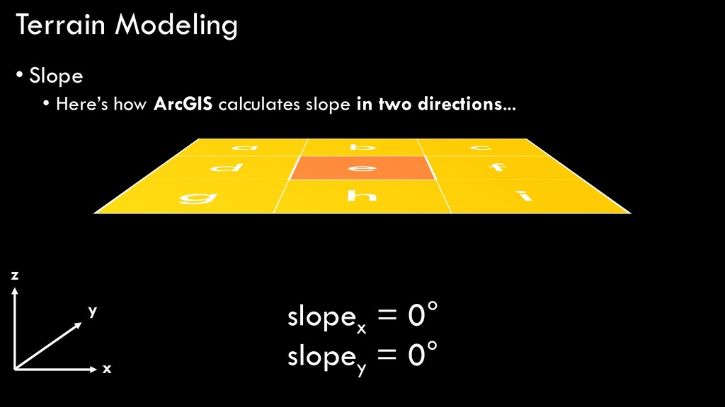
in two directions... • Uses a 3x3 focal neighborhood to calculate slope of the target cell a b c d e f g h i reference analysis window 3 x 3 neighborhood target analysis cell
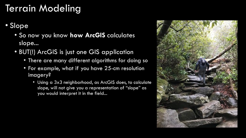
ArcGIS calculates slope... • BUT(!) ArcGIS is just one GIS application • There are many different algorithms for doing so • For example, what if you have 25-cm resolution imagery? • Using a 3x3 neighborhood, as ArcGIS does, to calculate slope, will not give you a representation of “slope” as you would interpret it in the field...
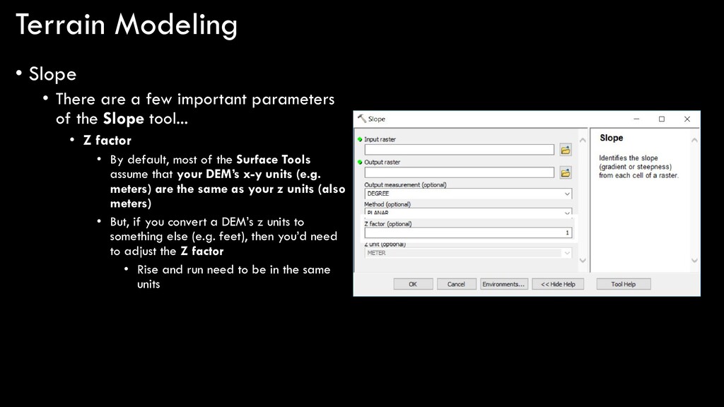
parameters of the Slope tool... • Z factor • By default, most of the Surface Tools assume that your DEM’s x-y units (e.g. meters) are the same as your z units (also meters) • But, if you convert a DEM’s z units to something else (e.g. feet), then you’d need to adjust the Z factor • Rise and run need to be in the same units
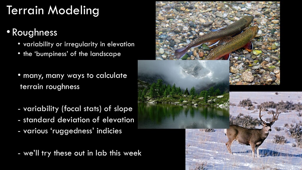
the ‘bumpiness’ of the landscape • many, many ways to calculate terrain roughness - variability (focal stats) of slope - standard deviation of elevation - various ‘ruggedness’ indicies - we’ll try these out in lab this week
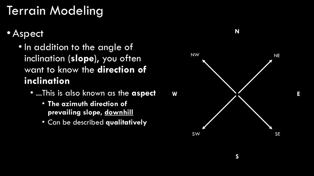
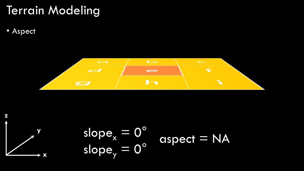
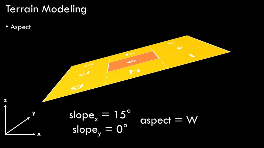
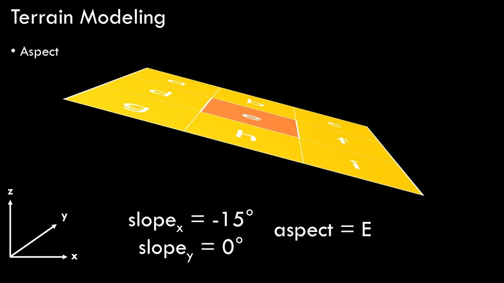
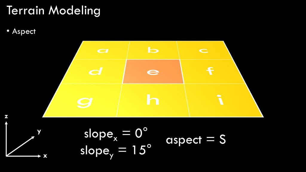
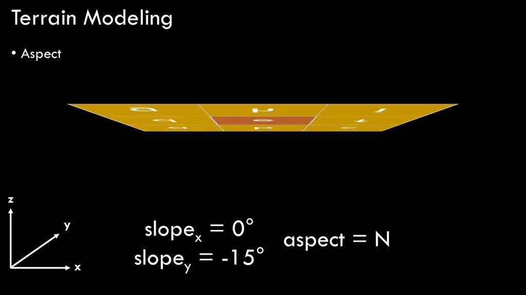
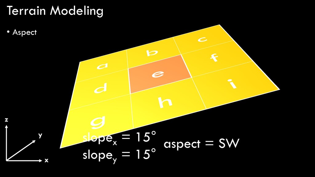
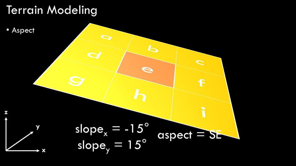
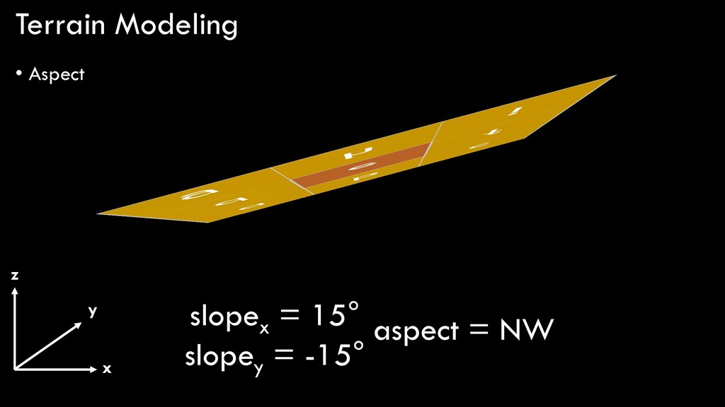
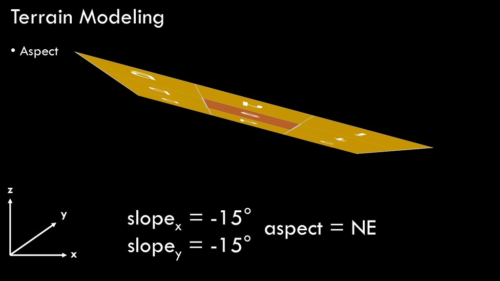
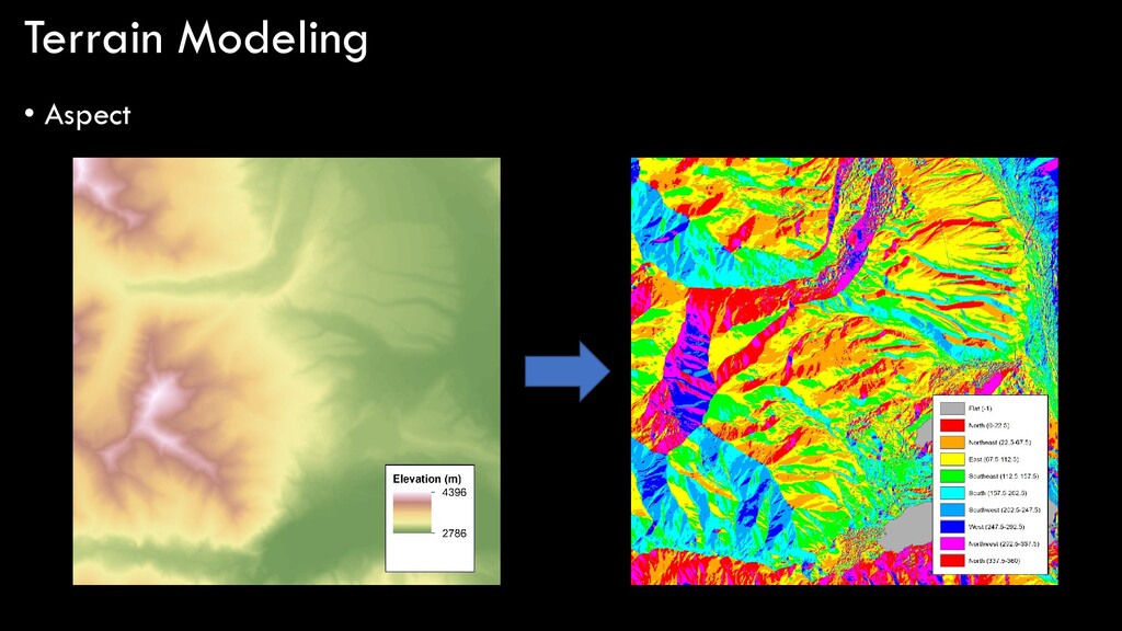
inclination (slope), you often want to know the direction of inclination • ...This is also known as the aspect • The azimuth direction of prevailing slope, downhill • Can be described qualitatively N E S W NE SE SW NW NNE ENE ESE SSE SSW WSW WNW NNW
inclination (slope), you often want to know the direction of inclination • ...This is also known as the aspect • The azimuthal direction of prevailing slope, downhill • Can be described qualitatively • Can also be described quantitatively 0°,360° 90° 180° 270° 45 ° 135° 225° 315 ° 22.5° 67.5° 112.5° 157.5° 202.5° 247.5° 292.5° 337.5°
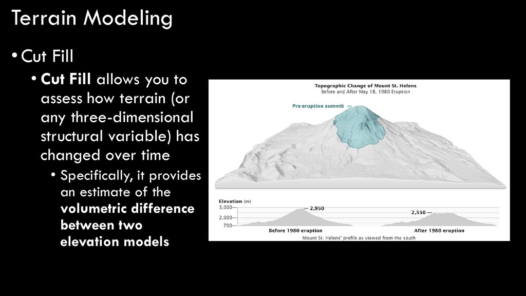
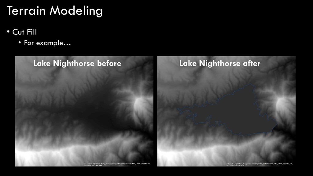
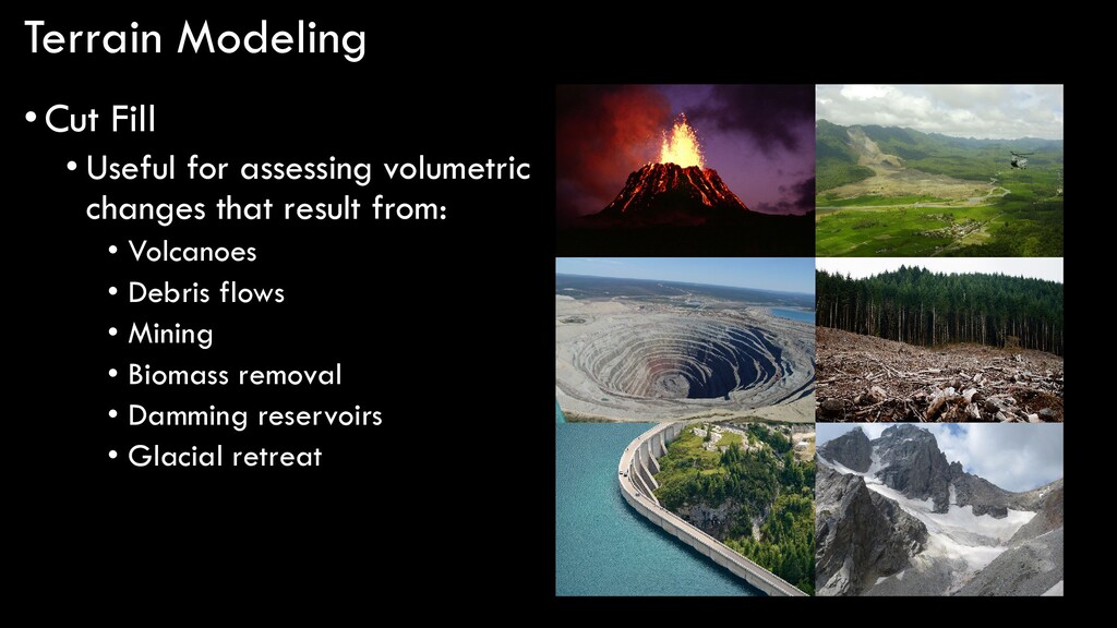
assess how terrain (or any three-dimensional structural variable) has changed over time • Specifically, it provides an estimate of the volumetric difference between two elevation models
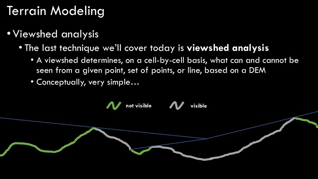
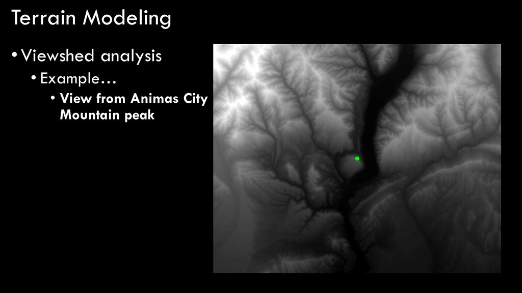
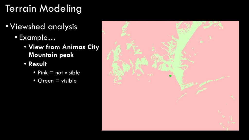
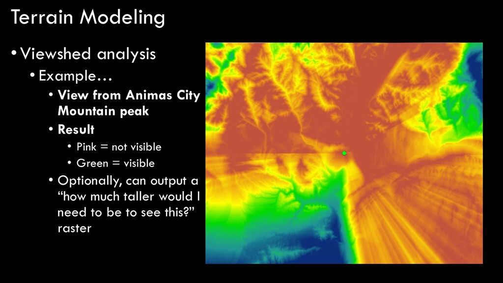
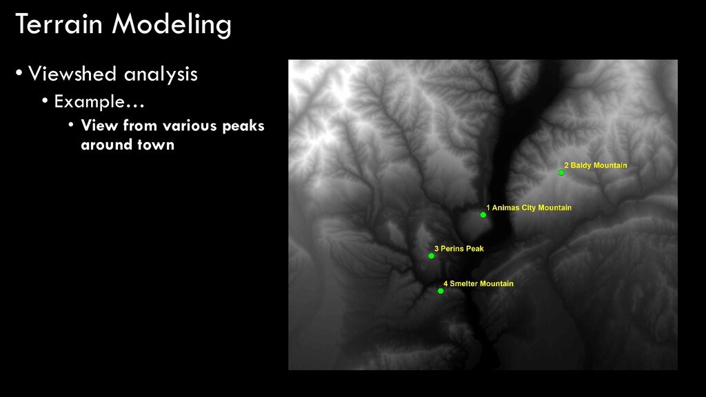
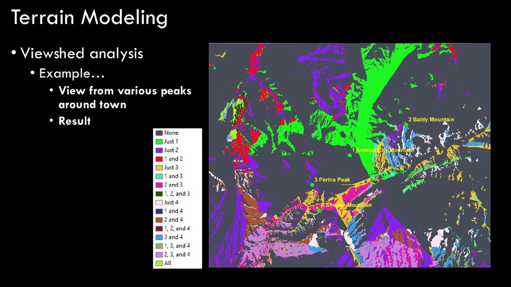
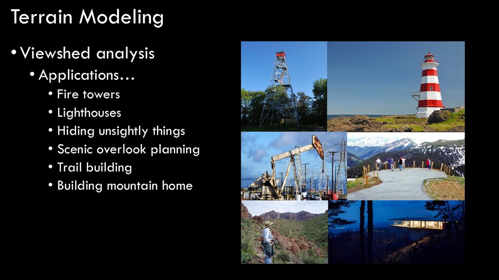
today is viewshed analysis • A viewshed determines, on a cell-by-cell basis, what can and cannot be seen from a given point, set of points, or line, based on a DEM • Conceptually, very simple… not visible visible
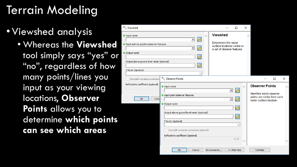
says “yes” or “no”, regardless of how many points/lines you input as your viewing locations, Observer Points allows you to determine which points can see which areas