CIDM Keynote Talk 2017

Transcript

1. Neyman-Pearson Feature Selection Sequential Learning for Subset Selection Online Learning and Feature Selection Applications of Feature Selection Scalable Feature Selections and Its Applications Gregory Ditzler The University of Arizona Department of Electrical & Computer Engineering ditzler@email.arizona.edu http://www2.engr.arizona.edu/˜ditzler CIDM Plenary Talk (28 Nov. 2017) Scalable Feature Selections and Its Applications
2. Neyman-Pearson Feature Selection Sequential Learning for Subset Selection Online Learning and Feature Selection Applications of Feature Selection Overview Plan of Attack for the Next 50 minutes 1 Overview of Large-Scale Subset Selection 2 Neyman-Pearson Feature Selection 3 Sequential Learning Subset Selection 4 Online Feature Selection 5 Applications & Conclusion CIDM Plenary Talk (28 Nov. 2017) Scalable Feature Selections and Its Applications
3. Neyman-Pearson Feature Selection Sequential Learning for Subset Selection Online Learning and Feature Selection Applications of Feature Selection Motivation Challenges and Constraints There are a lot of data being generated in today’s technological climate Pro: some data are useful Con: some data are not useful A little bit like finding the signal in the noise Some scenarios require that the variables maintain a physical interpretation e.g., life sciences and clinical tests Many data arrive in a stream. What if the process sampling from P(data, labels) is not fixed? Data aren’t small anymore What does it mean for data to be “big”? The five V’s: volume, velocity, variety, veracity, and value volume: number of observations and dimensionality velocity: data arrive in a stream value: not the cost, but the importance Twenty years of machine learning research has led to to a wide body of approaches for detecting value “volume” of 20 years ago is not the volume of today distributed, parallel, and statistically sound CIDM Plenary Talk (28 Nov. 2017) Scalable Feature Selections and Its Applications
4. Neyman-Pearson Feature Selection Sequential Learning for Subset Selection Online Learning and Feature Selection Applications of Feature Selection Feature Selection feature 1
 feature 2 .… feature 1
 feature 2 .… feature 1
 feature 2 .… x1 x2 xM 2 RK Feature Selection legitimate malicious legitimate y1 y2 yM x0 1 x0 2 x0 M 2 Rk Classification Knowledge
 Discovery Stick figures courtesy of xkcd.com Relevance, Weak Relevance
 and Irrelevance k < K y = (x) CIDM Plenary Talk (28 Nov. 2017) Scalable Feature Selections and Its Applications
5. Neyman-Pearson Feature Selection Sequential Learning for Subset Selection Online Learning and Feature Selection Applications of Feature Selection Related Works Wrapper Methods Find a subset of features F ⊂ X that provide a minimal loss with a classifier C. Typically provide a smaller loss on a data sets than embedded and filter-based feature selection methods. F may vary depending on the choice of the classifier. Examples: SVM-RFE, distributed wrappers, small loss + high complexity Embedded Methods Optimize the parameters of the classifier and the feature selection at the same time. θ∗ = arg min θ∈Θ {E[ (θ, D)] + Ω(θ)} = arg min θ∈Θ y − XTθ 2 2 s.t. θ 1 ≤ τ Examples: lasso, elastic-net, streamwise feature selection, online feature selection Filter Methods Find a subset of features F ⊂ X that maximize a function J that is not tied to classification loss (classifier independent). Generally faster than wrapper and embedded methods, but we cannot assume F will produce minimal loss. Examples: RELIEF, Cond. likelihood maximization, JMI CIDM Plenary Talk (28 Nov. 2017) Scalable Feature Selections and Its Applications
6. Neyman-Pearson Feature Selection Sequential Learning for Subset Selection Online Learning and Feature Selection Applications of Feature Selection Motivation Algorithm Description Experiments Neyman-Pearson Feature Selection CIDM Plenary Talk (28 Nov. 2017) Scalable Feature Selections and Its Applications
7. Neyman-Pearson Feature Selection Sequential Learning for Subset Selection Online Learning and Feature Selection Applications of Feature Selection Motivation Algorithm Description Experiments A Motivation Shortcomings with the State-of-the-Art How many features should be selected for any arbitrary filter function J(X), and what about noisy data? What if there are a large number of observations? Wrappers and embedded methods tie themselves to classifiers, which can make them overly complex and prone to overfitting. Not too many of those popular feature selection tools are built for large volumes of data. Proposed Solution (Neyman-Pearson Feature Selection – NPFS) NPFS was designed to scale a generic filter subset selection algorithm to large data, while detect with relevant set size from an initial condition independent of what a user feels is “relevant” working with the decisions of a base-selection algorithm Scalability is important, so NPFS models parallelism from a programatic perceptive Nicely fits into a MapReduce approach to parallelism How many parallel tasks does NPFS allow? How many slots are available? Concept: generate bootstrap data sets, perform feature selection, then reduce importance detections to a Neyman-Pearson hypothesis test CIDM Plenary Talk (28 Nov. 2017) Scalable Feature Selections and Its Applications
8. Neyman-Pearson Feature Selection Sequential Learning for Subset Selection Online Learning and Feature Selection Applications of Feature Selection Motivation Algorithm Description Experiments NPFS (in one figure) D Dataset Map D1 D2 Dn A (Dn , k) A (D2 , k) A (D1 , k) X:,2 X:,1 X:,n … 2 6 6 6 6 6 4 1 1 0 · · · 1 1 0 1 0 · · · 0 0 1 0 1 · · · 1 1 . . . . . . . . . ... . . . . . . 1 1 1 · · · 1 1 3 7 7 7 7 7 5 # features # of runs Reduce & Inference X i Xj,i ⇣crit ! ! if feature is relevant j X Λ(Z) = P(T(Z)|H1 ) P(T(Z)|H0 ) H1 ≷ H0 ζcrit → n z pz 1 (1 − p1 )n−z n z pz 0 (1 − p0 )n−z H1 ≷ H0 ζcrit α = P(T(Z) > ζcrit |H0 ) 1G. Ditzler, R. Polikar, and G. Rosen, “A bootstrap based Neyman-Pearson test for identifying variable importance,” IEEE Transactions on Neural Networks and Learning Systems, 2015, vol. 26, no. 4, pp. 880-886. 2G. Ditzler, M. Austen, R, Polikar, and G. Rosen, “Scalable Subset Selection and Variable Importance,” IEEE Symposium on Computational Intelligence in Data Mining, 2014. CIDM Plenary Talk (28 Nov. 2017) Scalable Feature Selections and Its Applications
9. Neyman-Pearson Feature Selection Sequential Learning for Subset Selection Online Learning and Feature Selection Applications of Feature Selection Motivation Algorithm Description Experiments The NPFS Algorithm NPFS Pseudo Code1 1 Run a FS algorithm A on n independently sampled data sets. Form a matrix X ∈ {0, 1}K×n where {X}il is the Bernoulli random variable for feature i on trial l. 2 Compute ζ crit using equation (1), which requires n, p0, and the Binomial inverse cumulative distribution function. P(z > ζ crit |H0) = 1 − P(z ≤ ζ crit |H0) cumulative distribution function = α (1) 3 Let {z}i = n l=1 {X}il. If {z}i > ζ crit then feature belongs in the relevant set; otherwise, the feature is deemed non-relevant. Concentration Inequality on |ˆ p − p| (Hoeffding’s bound) If X1, . . . , Xn ∼ Bernoulli(p), then for any > 0, we have P(|ˆ p − p| ≥ ) ≤ 2e−2n 2 where ˆ p = 1 n Zn. 3Matlab code is available. http://github.com/gditzler/NPFS. CIDM Plenary Talk (28 Nov. 2017) Scalable Feature Selections and Its Applications
10. Neyman-Pearson Feature Selection Sequential Learning for Subset Selection Online Learning and Feature Selection Applications of Feature Selection Motivation Algorithm Description Experiments Results on Synthetic Data 20 40 60 80 100 5 10 15 20 25 bootstrap feature (a) k = 10 20 40 60 80 100 5 10 15 20 25 bootstrap feature (b) k = 15 20 40 60 80 100 5 10 15 20 25 bootstrap feature (c) k = 20 20 40 60 80 100 5 10 15 20 25 bootstrap feature (d) k = 24 Figure: Visualization of X, where black segments indicate Xl = 0, white segments Xl = 1, and the orange rows are the features detected as relevant by NPFS. Note k∗ = 5. 0 100 200 300 400 500 0 5 10 15 20 25 number of bootstraps # features (max 50) k=3 k=5 k=10 k=15 k=25 (a) K = 50, k∗ = 15 0 100 200 300 400 500 0 5 10 15 20 25 number of bootstraps # features (max 100) k=3 k=5 k=10 k=15 k=25 (b) K = 100, k∗ = 15 0 100 200 300 400 500 0 10 20 30 40 number of bootstraps # features (max 250) k=3 k=5 k=10 k=15 k=25 (c) K = 250, k∗ = 15 Figure: Number of features selected by NPFS for varying levels of k. CIDM Plenary Talk (28 Nov. 2017) Scalable Feature Selections and Its Applications
11. Neyman-Pearson Feature Selection Sequential Learning for Subset Selection Online Learning and Feature Selection Applications of Feature Selection Motivation Algorithm Description Experiments Results on UCI Data data set |D| K nb nb-jmi nb-npfs cart cart-jmi cart-npfs breast 569 30 0.069 (3) 0.055 (1.5) 0.055 (1.5) 0.062 (3) 0.056 (2) 0.041 (1) congress 435 16 0.097 (3) 0.088 (1) 0.088 (2) 0.051 (3) 0.051 (1.5) 0.051 (1.5) heart 270 13 0.156 (1) 0.163 (2) 0.174 (3) 0.244 (3) 0.226 (2) 0.207 (1) ionosphere 351 34 0.117 (3) 0.091 (2) 0.091 (1) 0.077 (3) 0.068 (1) 0.074 (2) krvskp 3196 36 0.122 (3) 0.108 (1) 0.116 (2) 0.006 (1) 0.056 (3) 0.044 (2) landsat 6435 36 0.204 (1) 0.231 (2.5) 0.231 (2.5) 0.161 (1) 0.173 (2) 0.174 (3) lungcancer 32 56 0.617 (3) 0.525 (1) 0.617 (2) 0.542 (2) 0.558 (3) 0.533 (1) parkinsons 195 22 0.251 (3) 0.170 (1.5) 0.170 (1.5) 0.133 (1.5) 0.138 (3) 0.133 (1.5) pengcolon 62 2000 0.274 (3) 0.179 (2) 0.164 (1) 0.21 (1) 0.226 (2.5) 0.226 (2.5) pengleuk 72 7070 0.421 (3) 0.029 (1) 0.043 (2) 0.041 (2) 0.027 (1) 0.055 (3) penglung 73 325 0.107 (1) 0.368 (3) 0.229 (2) 0.337 (1) 0.530 (3) 0.504 (2) penglymp 96 4026 0.087 (1) 0.317 (3) 0.140 (2) 0.357 (3) 0.312 (2) 0.311 (1) pengnci9 60 9712 0.900 (3) 0.600 (2) 0.400 (1) 0.667 (2) 0.617 (1) 0.783 (3) semeion 1593 256 0.152 (1) 0.456 (3) 0.387 (2) 0.25 (1) 0.443 (3) 0.355 (2) sonar 208 60 0.294 (3) 0.279 (2) 0.241 (1) 0.259 (2) 0.263 (3) 0.201 (1) soybean 47 35 0.000 (2) 0.000 (2) 0.000 (2) 0.020 (2) 0.020 (2) 0.020 (2) spect 267 22 0.210 (2) 0.206 (1) 0.232 (3) 0.187 (1) 0.210 (2) 0.229 (3) splice 3175 60 0.044 (1) 0.054 (2) 0.055 (3) 0.085 (3) 0.070 (2) 0.066 (1) waveform 5000 40 0.207 (3) 0.204 (2) 0.202 (1) 0.259 (3) 0.238 (2) 0.228 (1) wine 178 13 0.039 (2.5) 0.039 (2.5) 0.034 (1) 0.079 (3) 0.068 (1.5) 0.068 (1.5) average 2.275 1.900 1.825 2.075 2.1250 1.800 Highlights CART+NPFS provides statistically significant improvement. NPFS (even after a large number of bootstraps) does not detect all features as important CIDM Plenary Talk (28 Nov. 2017) Scalable Feature Selections and Its Applications
12. Neyman-Pearson Feature Selection Sequential Learning for Subset Selection Online Learning and Feature Selection Applications of Feature Selection Motivation Algorithm Description Experiments Large Data Set Evaluation (53M+ observations) 100 200 300 400 500 600 0 100 200 300 400 500 600 data processed (MB) runtime (sec) LASSO NPFS (a) NPFS vs. LASSO 20 40 60 80 100 120 10 20 30 40 data processed (GB) runtime (min) NPFS (b) NPFS on Large Scale Data Figure: (left) Runtime of NPFS versus LASSO on a large synthetic dataset. (right) NPFS evaluated on a very large dataset. The NPFS times can be interpreted as the amount of time it takes to complete a dataset of size XGB. CIDM Plenary Talk (28 Nov. 2017) Scalable Feature Selections and Its Applications
13. Neyman-Pearson Feature Selection Sequential Learning for Subset Selection Online Learning and Feature Selection Applications of Feature Selection Motivation Algorithm Description Experiments Sequential Learning for Subset Selection CIDM Plenary Talk (28 Nov. 2017) Scalable Feature Selections and Its Applications
14. Neyman-Pearson Feature Selection Sequential Learning for Subset Selection Online Learning and Feature Selection Applications of Feature Selection Motivation Algorithm Description Experiments Sequential Learning for Subset Selection (SLSS) Motivation NPFS is an elegant and effective approach for inferring k∗ with any generic subset selection algorithm (A) that returns k of K features; however, NPFS uses A to evaluate all feature variables at each iteration. This evaluation could be too computationally intensive Smaller problems are ∗generally∗ easier to solve than larger ones. Motivation for Bandits and Sequential Learning The multi-arm bandit (MAB) addresses the problem of exploration-versus-exploitation (EvE) when a player needs to select a decision (from one of many) that maximizes the reward of the player over time. In our setting, a player must select a feature subset to maximize their reward. We propose a bandit-like approach to explore the combinatorial search space and return an importance distribution over the features 1G. Ditzler, R. Polikar, and G. Rosen, “Sequential decision processes for feature subset selection and relevancy ranking,” IEEE Transactions on Neural Networks and Learning Systems, 2017. In Press. CIDM Plenary Talk (28 Nov. 2017) Scalable Feature Selections and Its Applications
15. http://www.fingerlakesgaming.com/styles/Slots(1).jpg feature 1 feature 2 feature 3 feature 4 feature 8 feature 7 feature 6 feature 5 feature 9 feature 11 feature 10 $$$$ = reward
16. Neyman-Pearson Feature Selection Sequential Learning for Subset Selection Online Learning and Feature Selection Applications of Feature Selection Motivation Algorithm Description Experiments Pseudo code for two SLSS implementations input data D, number of rounds T, number of features k selected by A, subset size , and weak reward η ∈ [0, 1]. Initialize: Tj , rj = 0 for j ∈ [K] and set weights w1 j = 0 for j ∈ [K] Pure Exploration: Explore all features using subsets of size until all features have been tested (i.e., Tj > 0). 1: for t = 1, . . . , T do 2: Choose largest features from wt j = wt j + 2 log t Tj Refer to this set of indices as Kt. 3: It = A(D(Kt), k) 4: Tj ← Tj + 1 for j ∈ Kt 5: rj ← rj + 1 for j ∈ It 6: rj ← rj + η for j ∈ Kt \It 7: Update weights wt+1 j for j ∈ Kt 8: end for input data D, rounds T, number of features k selected by A, , η ∈ [0, 1] and γ ∈ [0, 1]. Initialize: Tj , rj = 0 for j ∈ [K] and set weights w1 j = 0 for j ∈ [K] Pure Exploration 1: for t = 1, . . . , T do 2: Choose largest features from pj = (1 − γ) wt j K i=1 wt i + γ K Refer to this set of indices as Kt. 3: It = A(D(Kt), k) 4: rj ← rj + 1 for j ∈ It 5: rj ← rj + η for j ∈ Kt \It 6: Set: wt+1 j = wt j exp        γ rt j        7: end for CIDM Plenary Talk (28 Nov. 2017) Scalable Feature Selections and Its Applications
17. Neyman-Pearson Feature Selection Sequential Learning for Subset Selection Online Learning and Feature Selection Applications of Feature Selection Motivation Algorithm Description Experiments High-level overview of SLSS Leveraging Exploration & Exploitation SLSS is a framework for feature selection with partial inputs that uses 4 different bandits (UCB1, -greedy, Exp3, Thompson) Completely classifier-independent unlike previous attempts for performing feature selection with bandits SLSS learns a set of “importance” weights over the features Selecting Features Unlike NPFS, SLSS does not immediately return the relevant feature set, rather it returns a set of weights. SLSS uses a sampling procedure to go from the weights to the relevant feature set Input: data set D, a base subset selection method A, importance weights w ∈ [0, 1]K , and a bandit B. 1 B selects q of K features using w 2 A evaluates and is given a set of reward for the q features 3 Update weights w using the rewards 4 Repeat until convergence in w input SLSS feature weights w, and number of simulations M. 1: for m = 1, . . . , M do 2: Choose Qm as a random sample of [K] using w 3: k∗ m = Unique(Qm) 4: end for output Size of feature importance set ˆ k∗ =           1 M M m=1 k∗ m           CIDM Plenary Talk (28 Nov. 2017) Scalable Feature Selections and Its Applications
18. Neyman-Pearson Feature Selection Sequential Learning for Subset Selection Online Learning and Feature Selection Applications of Feature Selection Motivation Algorithm Description Experiments SLSS Weight Evolution as a function of T (a) SLSS-Exp3 (b) SLSS- (c) SLSS-Thom (d) SLSS-UCB1 (e) SLSS-Exp3 (sig.) (f) SLSS- (sig.) (g) SLSS-Thom (sig.) (h) SLSS-UCB1 (sig.) CIDM Plenary Talk (28 Nov. 2017) Scalable Feature Selections and Its Applications
19. Neyman-Pearson Feature Selection Sequential Learning for Subset Selection Online Learning and Feature Selection Applications of Feature Selection Motivation Algorithm Description Experiments Results on real-world data Table: Properties of data sets used in our experiments. data set instances features Caporaso 467 1193 American Gut 2905 3110 Colon 62 2000 Lung 73 325 NCI9 60 9712 Leuk 72 7070 Sido0 12678 4932 Table: Rank of an algorithm’s performance when averaged across the data sets (lower is better). 5-NN CART algorithm error f1 error f1 Base 6.21 5.86 5.86 6.57 MIM 4.93 4.00 5.21 4.14 mRMR 6.21 4.93 3.50 4.29 NPFS 5.14 6.14 5.86 5.43 SLSS-UCB1 3.71 4.79 3.00 3.57 SLSS-Thom 2.36 2.93 3.50 4.14 SLSS- 3.29 3.43 3.50 2.14 SLSS-Exp3 4.14 3.93 5.57 5.71 Results For the 5-NN, we find that the Friedman test rejects the null hypothesis that the error rates are equal; however, there is not enough statistical significance to state there is a difference in the f1-measure. For CART, significant improvements are observed with the error of SLSS-UCB1 (base, MIM and NPFS), SLSS-Thompson (base and NPFS), and SLSS- (base). CIDM Plenary Talk (28 Nov. 2017) Scalable Feature Selections and Its Applications
20. Neyman-Pearson Feature Selection Sequential Learning for Subset Selection Online Learning and Feature Selection Applications of Feature Selection Motivation Algorithm Description Experiments SLSS Evaluated with the Bag-of-Little Bootstraps 0 1000 2000 3000 4000 time (seconds) 0.115 0.12 0.125 0.13 0.135 0.14 Error SLSS SLSS-BLB CIDM Plenary Talk (28 Nov. 2017) Scalable Feature Selections and Its Applications
21. Neyman-Pearson Feature Selection Sequential Learning for Subset Selection Online Learning and Feature Selection Applications of Feature Selection Concept Drift Online Learning Ensembles Experiments Online Learning and Feature Selection CIDM Plenary Talk (28 Nov. 2017) Scalable Feature Selections and Its Applications
22. Neyman-Pearson Feature Selection Sequential Learning for Subset Selection Online Learning and Feature Selection Applications of Feature Selection Concept Drift Online Learning Ensembles Experiments Concept Drift & Multiple Experts Concept drift Concept drift can be modeled as a change in a probability distribution, P(X, Ω). The change can be in P(X), P(X|Ω), P(Ω), or joint changes in P(Ω|X). P(Ω|X) = P(X|Ω)P(Ω) P(X) We generally reserve names for specific types of drift (e.g., real and virtual) Drift types: sudden, gradual, incremental, & reoccurring General Examples: electricity demand, financial, climate, epidemiological, and spam (to name a few) 0 5 10 15 20 25 0 0.1 0.2 0.3 0.4 0.5 0.6 0.7 dα/dt time Constant Sinusoidal Exponential Incremental Learning Incremental learning can be summarized as the preservation of old knowledge without access to old data. Desired concept drift algorithm should find a balance between prior knowledge (stability) and new knowledge (plasticity). . . Stability-Plasticity Dilemma Ensembles have been shown to provide a good balance between stability and plasticity CIDM Plenary Talk (28 Nov. 2017) Scalable Feature Selections and Its Applications
23. Neyman-Pearson Feature Selection Sequential Learning for Subset Selection Online Learning and Feature Selection Applications of Feature Selection Concept Drift Online Learning Ensembles Experiments Concept Drift & Multiple Experts Incremental Learning Procedure Train Expert ht Update Weights Predict St+1 Measure (H, ft+1) S1 , . . . , St (H, ft+1) H(x) = t k=1 wk,thk(x) ⇒ H = t k=1 wk,thk and ˆ y = sign(H) Algorithms that follow this setting (more or less): Learn++.NSE, SERA, SEA, DWM, . . . 1G. Ditzler, M. Roveri, C. Alippi, and R. Polikar, “Adaptive strategies for learning in nonstationary environments: a survey,” IEEE Computational Intelligence Magazine, 2015, vol. 10, no. 4, pp. 12–25. CIDM Plenary Talk (28 Nov. 2017) Scalable Feature Selections and Its Applications
24. Neyman-Pearson Feature Selection Sequential Learning for Subset Selection Online Learning and Feature Selection Applications of Feature Selection Concept Drift Online Learning Ensembles Experiments Online Feature Selection Overview Previous approaches were classifier-independent; however, there are advantages to other approaches such as embedded Easy to account for correlations between many features Improvements to optimization benefit embedded approaches Easy to adapt to drifting probability distributions1 An ensemble of classifiers can be used to reduce the error rate in incremental learning scenarios2, though there can be an increased complexity. Contribution Build an ensemble of classifiers that can learn from partial information, and perform feature selection simultaneously. A linear B-sparse model ( w 0 ≤ B for a model w) for an ensemble yields lower error rates than a B-sparse single model. The ensemble is the same complexity of a single model at the time of classification. 1G. Ditzler, M. Roveri, C. Alippi, and R. Polikar, “Adaptive strategies for learning in nonstationary environments: a survey,” IEEE Computational Intelligence Magazine, 2015, vol. 10, no. 4, pp. 12–25. 2G. Ditzler, G. Rosen, and R. Polikar, “Domain Adaptation Bounds for Multiple Expert Systems Under Concept Drift,” International Joint Conference on Neural Networks, 2014. (best student paper award) CIDM Plenary Talk (28 Nov. 2017) Scalable Feature Selections and Its Applications
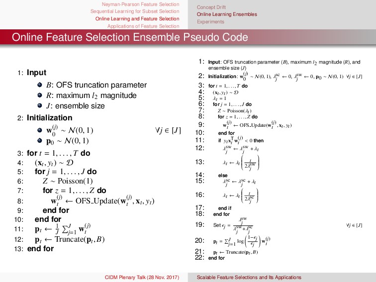
25. Neyman-Pearson Feature Selection Sequential Learning for Subset Selection Online Learning and Feature Selection Applications of Feature Selection Concept Drift Online Learning Ensembles Experiments Online Feature Selection Ensemble Pseudo Code 1: Input B: OFS truncation parameter R: maximum l2 magnitude J: ensemble size 2: Initialization w(j) 0 ∼ N(0, 1) ∀j ∈ [J] p0 ∼ N(0, 1) 3: for t = 1, . . . , T do 4: (xt , yt) ∼ D 5: for j = 1, . . . , J do 6: Z ∼ Poisson(1) 7: for z = 1, . . . , Z do 8: w(j) t ← OFS Update(w(j) t , xt , yt) 9: end for 10: end for 11: pt ← 1 J J j=1 w(j) t 12: pt ← Truncate(pt , B) 13: end for 1: Input: OFS truncation parameter (B), maximum l2 magnitude (R), and ensemble size (J) 2: Initialization: w (j) 0 ∼ N(0, 1), λsc j ← 0, λsw j ← 0, p0 ∼ N(0, 1) ∀j ∈ [J] 3: for t = 1, . . . , T do 4: (xt, yt) ∼ D 5: λt = 1 6: for j = 1, . . . , J do 7: Z ∼ Poisson(λt) 8: for z = 1, . . . , Z do 9: w (j) t ← OFS Update(w (j) t , xt, yt) 10: end for 11: if ytxT t w (j) t < 0 then 12: λsw j ← λsw j + λt 13: λt ← λt         t 2λsw j         14: else 15: λsc j ← λsc j + λt 16: λt ← λt         t 2λsc j         17: end if 18: end for 19: Set j = λsw j λsw j +λsc j ∀j ∈ [J] 20: pt = J j=1 log 1− j j w (j) t 21: pt ← Truncate(pt, B) 22: end for CIDM Plenary Talk (28 Nov. 2017) Scalable Feature Selections and Its Applications
26. Neyman-Pearson Feature Selection Sequential Learning for Subset Selection Online Learning and Feature Selection Applications of Feature Selection Concept Drift Online Learning Ensembles Experiments Learning Setting & Contribution Online Learning Data arrive one instance at a time and are only available at the time they’re presented 3 of the 5 V’s: Volume, Velocity and Value Pro/Con Pro: Update classifier parameters without a batch update Con: Typically learns slower than a batch algorithm Contribution Two variations of online bagging and boosting using existing linear models for learning with partial information Ensemble model is B-sparse and typically results in lower error rates Input Distribution D, learning rule Update, parameter vector w ∼ N(0, 1)K×1 for t = 1, 2, . . . 1 Receive (xt , yt) ∼ D 2 Update w = Update(w, xt , yt) 3 Receive test instance x ∼ D 4 Receive y and measure the loss (wTx, y) 1G. Ditzler, J. LaBarck, G. Rosen, and R. Polikar, “Improvements to Scalable Online Feature Selection Using Bagging and Boosting,” IEEE Transactions on Neural Networks and Learning Systems, 2017. In Press. CIDM Plenary Talk (28 Nov. 2017) Scalable Feature Selections and Its Applications
27. Neyman-Pearson Feature Selection Sequential Learning for Subset Selection Online Learning and Feature Selection Applications of Feature Selection Concept Drift Online Learning Ensembles Experiments A Note About Diversity Diversity, Diversity, and Diversity! Diversity, specifically diversity within the single classifiers, is generally a preferred quality for an ensemble Why use an ensemble if the single models all predict the same thing? Promoting diversity tends to lead better error rates, though the connection between error and diversity is not trivial. Diversity can be controlled using several different techniques Bootstrap samples then bootstrap features (random forests) Set different free parameters for each base classifier Diversity in OFSE Let B be a random variable sampled from Poisson(λ) e.g., λ = βK for β ∈ (0, 1) 0 20 40 60 80 100 0 0.05 0.1 0.15 0.2 0.25 0.3 0.35 0.4 B pdf λ=1 λ=10 λ=25 λ=50 CIDM Plenary Talk (28 Nov. 2017) Scalable Feature Selections and Its Applications
28. Neyman-Pearson Feature Selection Sequential Learning for Subset Selection Online Learning and Feature Selection Applications of Feature Selection Concept Drift Online Learning Ensembles Experiments Summary of UCI Experiments Testing for Significance The Friedman rank test rejects the hypothesis that all algorithms are performing equally (pF = 5.6738 × 10−12) All ensemble approaches outperform the single model with statistical significance (α/4 indicates significance) Conclusions Only a portion of the features are required (B) for learning, and each each single model performs feature selection The ensemble consistently outperforms the single model Single OBag OBoo OBag-R OBoo-R Single – 0.9997 1.0000 0.9998 1.0000 OBag 0.0003 – 0.9532 0.5445 0.9873 OBoo 0.0000 0.0468 – 0.0588 0.7119 OBag-R 0.0002 0.4555 0.9412 – 0.9832 OBoo-R 0.0000 0.0127 0.2881 0.0168 – p-values from the Bonferroni-Dunn test (see Demˇ sar (2006)) CIDM Plenary Talk (28 Nov. 2017) Scalable Feature Selections and Its Applications
29. Neyman-Pearson Feature Selection Sequential Learning for Subset Selection Online Learning and Feature Selection Applications of Feature Selection Fizzy: Feature Selection for Metagenomics Adversarial Machine Learning and Feature Selection Filina Applications of Feature Selection: The Microbiome CIDM Plenary Talk (28 Nov. 2017) Scalable Feature Selections and Its Applications
31. Functional Composition! Taxonomic Composition! Who is there? How much of them are there? ! What are their functions?!
32. Functional Composition! Taxonomic Composition! Unhealthy! vs.! Healthy !
34. Neyman-Pearson Feature Selection Sequential Learning for Subset Selection Online Learning and Feature Selection Applications of Feature Selection Fizzy: Feature Selection for Metagenomics Adversarial Machine Learning and Feature Selection Filina Overview of Feature Selection with Biological Data Measure Abundance Functional Databases (Pfam, SEED, etc.) Abundance Profile Fizzy Frequencies of Selected Variables and Interpretation Training Metagenomes Group 1 Group 2 Testing Metagenomes Classify Train Classifier Measure loss and determine feature subsets that have lowest loss and highest AUC User Supplied Why another software tool? Feature selection has become increasingly popular, yet the vast majority of tools are classifier-dependent Provide complementary support to β-diversity analysis Software Flow Overview Compatible with commonly used biological data formats Built on top of the FEAST C library Biom File Sparse/dense representation of the OTU table in JSON format. Map File Meta-data corresponding to the Biom file. One column contains the class labels for the Biom file. Parameters Parameters for feature selection. Output File path to save the OTU IDs of the relevant features. Fizzy Suite Feature Selection lasso PyFeast Post-Processing Fizzy NPFS 1G. Ditzler, J. Calvin Morrison, Y. Lan, and G. Rosen, “Fizzy: Feature selection for metagenomics,” BMC Bioinformatics, 2015, vol 16, no. 358. CIDM Plenary Talk (28 Nov. 2017) Scalable Feature Selections and Its Applications
35. Neyman-Pearson Feature Selection Sequential Learning for Subset Selection Online Learning and Feature Selection Applications of Feature Selection Fizzy: Feature Selection for Metagenomics Adversarial Machine Learning and Feature Selection Filina Metahit: A study of patients with and without IBD List of the top five ranked Pfams as selected by the Fizzy’s Mutual Information Maximization (MIM) applied to MetaHit Rank IBD features F1 ABC transporter (PF00005) F2 Phage integrase family (PF00589) F3 Glycosyl transferase family 2 (PF00535) F4 Acetyltransferase (GNAT) family (PF00583) F5 Helix-turn-helix (PF01381) Rank Obese features F1 ABC transporter (PF00005) F2 MatE (PF01554) F3 TonB dependent receptor (PF00593) F4 Histidine kinase-, DNA gyrase B-, and HSP90-like ATPase (PF02518) F5 Response regulator receiver domain (PF00072) Interpreting the results Glycosyl transferase (PF00535) was selected by MIM, furthermore, its alternation is hypothesized to result in recruitment of bacteria to the gut mucosa and increased inflammation A genotype of acetyltransferase (PF00583) plays an important role in the pathogenesis of IBD ATPases (PF02518) catalyze dephosphorylation reactions to release energy 0 200 400 600 800 1000 0 100 200 300 400 500 Selected Features Time (seconds) JMI mRMR MIM Lasso NPFS−MIM RFC 1G. Ditzler, Y. Lan, J.-L. Bouchot, and G. Rosen, “Feature selection for metagenomic data analysis,” Encyclopedia of Metagenomics, 2014. CIDM Plenary Talk (28 Nov. 2017) Scalable Feature Selections and Its Applications
36. Neyman-Pearson Feature Selection Sequential Learning for Subset Selection Online Learning and Feature Selection Applications of Feature Selection Fizzy: Feature Selection for Metagenomics Adversarial Machine Learning and Feature Selection Filina Applications of Feature Selection: Adversarial Learning CIDM Plenary Talk (28 Nov. 2017) Scalable Feature Selections and Its Applications
37. Neyman-Pearson Feature Selection Sequential Learning for Subset Selection Online Learning and Feature Selection Applications of Feature Selection Fizzy: Feature Selection for Metagenomics Adversarial Machine Learning and Feature Selection Filina Feature Selection feature 1
 feature 2 .… feature 1
 feature 2 .… feature 1
 feature 2 .… x1 x2 xM 2 RK Feature Selection legitimate malicious legitimate y1 y2 yM x0 1 x0 2 x0 M 2 Rk Classification Knowledge
 Discovery Stick figures courtesy of xkcd.com Relevance, Weak Relevance
 and Irrelevance k < K y = (x) Adversary Abilities Poison: Adversary inserts/deletes/manipulates samples at training time to thwart the objective of a learning algorithm Evasion: Adversary manipulates malicious samples at evaluation time to attempt to come off as legitimate CIDM Plenary Talk (28 Nov. 2017) Scalable Feature Selections and Its Applications
38. Neyman-Pearson Feature Selection Sequential Learning for Subset Selection Online Learning and Feature Selection Applications of Feature Selection Fizzy: Feature Selection for Metagenomics Adversarial Machine Learning and Feature Selection Filina Feature Selection x1 x2 xM 2 RK legitimate malicious legitimate y1 y2 yM Stick figures courtesy of xkcd.com I know what you’re using b y legitimate? malicious? f(x) Adversary Abilities Poison: Adversary inserts/deletes/manipulates samples at training time to thwart the objective of a learning algorithm Evasion: Adversary manipulates malicious samples at evaluation time to attempt to come off as legitimate CIDM Plenary Talk (28 Nov. 2017) Scalable Feature Selections and Its Applications
39. Neyman-Pearson Feature Selection Sequential Learning for Subset Selection Online Learning and Feature Selection Applications of Feature Selection Fizzy: Feature Selection for Metagenomics Adversarial Machine Learning and Feature Selection Filina Learning in the Presence of an Adversary Is Feature Selection Secure? Attacker’s goal is to maximally increase the classification error of methods such as LASSO, Elastic Nets and Ridge Regression Xiao et al. provided a framework to essentially “break” LASSO by adding in a few new data samples into the training data, such that D := D ∪ xc max xc 1 2m m i=1 (yi − θTxi)2 + λ p j=1 |θj | The adversary has access to λ and the training data, which could be a bit far reaching assumption Acts as a wrapper to LASSO by finding xc via a (sub)gradient-ascent algorithm Impacts LASSO-based feature selection is quite susceptible to a meticulously carried out attack LASSO can be broken! How can we fix it? 0 0.05 0.1 0.15 0.2 % Poison 0.15 0.2 0.25 0.3 0.35 Error p=150 p=200 p=250 p=300 1H. Xiao et al., “Is feature selection secure against training data poisoning?,” ICML, 2015. CIDM Plenary Talk (28 Nov. 2017) Scalable Feature Selections and Its Applications
40. Neyman-Pearson Feature Selection Sequential Learning for Subset Selection Online Learning and Feature Selection Applications of Feature Selection Fizzy: Feature Selection for Metagenomics Adversarial Machine Learning and Feature Selection Filina Adversarial Machine Learning and Feature Selection A Wrapper Method Previous work has focused on devising adversary-aware classification algorithms to counter evasion attempts. No work has been considered with the problem of learning secure feature selection-based classifiers against evasion attacks Zhang et al. introduced a wrapper for feature selection 1: Input: x: the malicious sample; x(0): the initial location of the attack sample; η: step size; : small positive const.; m: max. iterations. 2: i = 1 3: while c(x(i), x) − c(x(i−1), x) < or i ≥ m do 4: if g(x(i)) ≥ 0 then 5: x(i) = x(i−1) − η∇g(x(i−1)) 6: else 7: x(i) = x(i−1) − η∇c(x(i−1), x) 8: end if 9: end while 1F. Zhang et al., “Adversarial feature selection against evasion attacks,” IEEE Transactions on Cybernetics, 2016. CIDM Plenary Talk (28 Nov. 2017) Scalable Feature Selections and Its Applications
41. Neyman-Pearson Feature Selection Sequential Learning for Subset Selection Online Learning and Feature Selection Applications of Feature Selection Fizzy: Feature Selection for Metagenomics Adversarial Machine Learning and Feature Selection Filina Preliminaries What going on with the Adversary? We are provided training data that we can assume is i.i.d. from a source domain DS. The test data are sampled from a target DT , such that kl(DS , DT ) > 0. The adversary controls the target domain, DT , by causing perturbations Divergences and Bounds on Learning The H∆H distance measures the maximum difference in expected loss between h, h ∈ H, on two distributions (Kifer et al.) dH∆H (DT , Dk) = 2 sup h,h ∈H |ET [ (h, h )] − Ek[ (h, h )]| Ben-David et al. bounded the loss of a single hypothesis being evaluated on an unknown distribution. ET (h, fT ) ≤ ES (h, f) + λ + 1 2 dH∆H (UT , US) 0 5 10 x 105 0 0.5 1 1.5 2 2.5 3 N VC confidence ν=100 ν=200 ν=500 ν=5000 CIDM Plenary Talk (28 Nov. 2017) Scalable Feature Selections and Its Applications
42. Neyman-Pearson Feature Selection Sequential Learning for Subset Selection Online Learning and Feature Selection Applications of Feature Selection Fizzy: Feature Selection for Metagenomics Adversarial Machine Learning and Feature Selection Filina Thinking Out Loud A Glimpse at the Error Ultimately, we are interested in knowing what the error of h will be on the target domain (i.e., legitimate, malicious, evasive-malicious) ET (h, fT ) ≤ ES (h, fS) Training Error + Divergence on Distributions 1 2 dH∆H (UT , US) + ES (h∗, fS) + ET (h∗, fT ) Terms needs to be taken into account, but an adversary doesn’t give it up where h∗ = arg min ES (h∗, fS) + ET (h∗, fT ) . What would we like to do? LASSO minimizes the sum-squared error and the L1-norm of θ; however, we want to examine a modified objective that tunes the model with adversarial information: θ∗ = arg min β∈Φ              (θ, D) model loss + regularization λΩ(θ) + αΛ(θ, D) adversary              where λ, α > 0 are regularization parameters that control the weight tied to the complexity and adversary, respectfully. What does Λ look like? Ideally convex? CIDM Plenary Talk (28 Nov. 2017) Scalable Feature Selections and Its Applications
43. Neyman-Pearson Feature Selection Sequential Learning for Subset Selection Online Learning and Feature Selection Applications of Feature Selection Fizzy: Feature Selection for Metagenomics Adversarial Machine Learning and Feature Selection Filina A Modified Objective What do we know? There are “textbook” attack strategies for families of classifiers and the degree of impact is controlled by the knowledge the adversary has about the classifier The attacker would likely only be interested in evasion at evaluation time, so causing maximum damage is generally not the objective Given positive (+) data, we can generate evasion sample Modifying the Objective Function In the spirit of LASSO and the Elastic net, add in a new (convex term) that is meant to “fine tune” the classifier and feature selector for possible evasions based on a known malicious sample. θ = arg min β∈Φ 1 2n n i=1 (yi − θTxi)2 + λ p j=1 |θj| + α 2m m i=1 (yi − θTxi)2 where xi are evasion samples and yi = +1. CIDM Plenary Talk (28 Nov. 2017) Scalable Feature Selections and Its Applications
44. Neyman-Pearson Feature Selection Sequential Learning for Subset Selection Online Learning and Feature Selection Applications of Feature Selection Fizzy: Feature Selection for Metagenomics Adversarial Machine Learning and Feature Selection Filina A Perfect Adversary? err = 1 m m i=1 sign(yi ) sign(θTxi ) , err · 0 = θ 0 , err · 2 2 = θ∗ − θ 2 2 θ∗ 2 2 Table: Classification error, model error, sparsity and evaluation time for LASSO, LASSO-RL and a game-theoretic approach. Original DS Evasion DT LASSO LASSO-RL GAME LASSO LASSO-RL GAME err 0.181 0.182 0.248 0.2904 0.22472 0.15962 err · 2 2 0.551 0.559 0.716 – – – err · 0 36.48 32.98 48.5 – – – AUC 0.88 0.87 0.81 – – – Time (s) 0.38 11.54 23.86 – – – Take Away Examining a worst-case adversary has negative effects on the classification error LASSO-RL provides a middle ground between LASSO and the game-theoretic approach Wrapper-based feature selection approaches are generally computationally burdensome (and this is not a large data set) CIDM Plenary Talk (28 Nov. 2017) Scalable Feature Selections and Its Applications
45. Neyman-Pearson Feature Selection Sequential Learning for Subset Selection Online Learning and Feature Selection Applications of Feature Selection Fizzy: Feature Selection for Metagenomics Adversarial Machine Learning and Feature Selection Filina Summary Take Away Feature section remains a part of nearly to nearly all data science pipelines and is often omitted in many conversations, despite it being there. Data are not small anymore! The era of big data not only is concerned with the volume of the data, but also the dimensionality of each of the data samples. There are many application driven fields that provide the field of feature selection with new challenges that are both practical and theoretical. CIDM Plenary Talk (28 Nov. 2017) Scalable Feature Selections and Its Applications
46. Neyman-Pearson Feature Selection Sequential Learning for Subset Selection Online Learning and Feature Selection Applications of Feature Selection Fizzy: Feature Selection for Metagenomics Adversarial Machine Learning and Feature Selection Filina Questions? CIDM Plenary Talk (28 Nov. 2017) Scalable Feature Selections and Its Applications