Lecture slides for POM 1-3

生産管理技術1の講義3のスライドです．

Transcript

1. © Hajime Mizuyama Production & Operations Management #1 @AGU Lec.3: Outline of Production Management (2) • MTS and MTO production • Demand forecasting and production planning • Planning and control of production
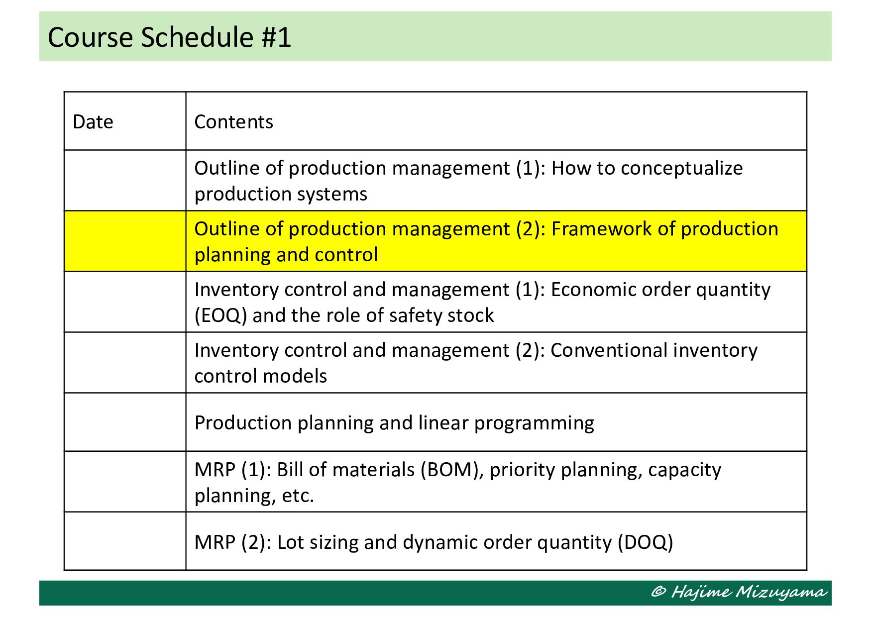
2. © Hajime Mizuyama Course Schedule #1 Date Contents Outline of production management (1): How to conceptualize production systems Outline of production management (2): Framework of production planning and control Inventory control and management (1): Economic order quantity (EOQ) and the role of safety stock Inventory control and management (2): Conventional inventory control models Production planning and linear programming MRP (1): Bill of materials (BOM), priority planning, capacity planning, etc. MRP (2): Lot sizing and dynamic order quantity (DOQ)
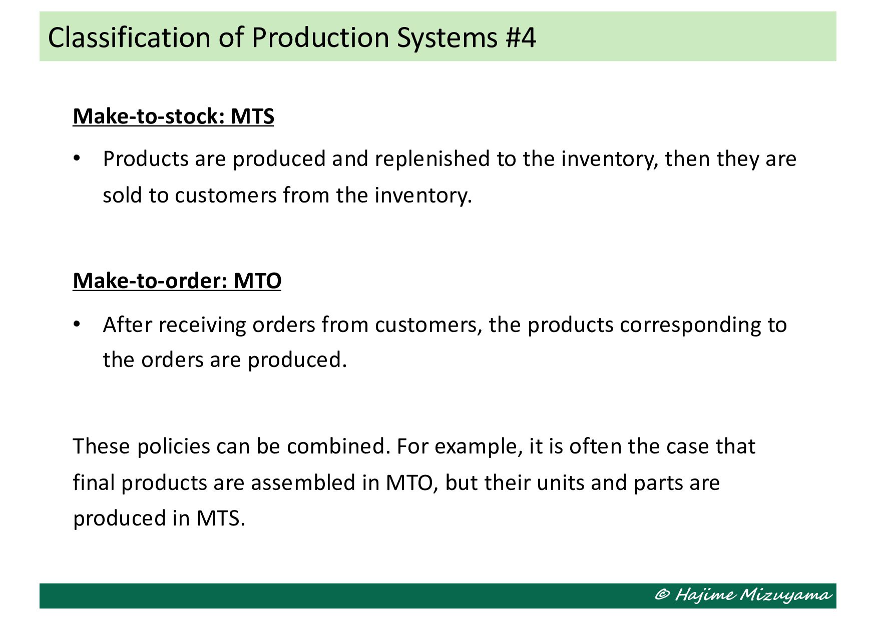
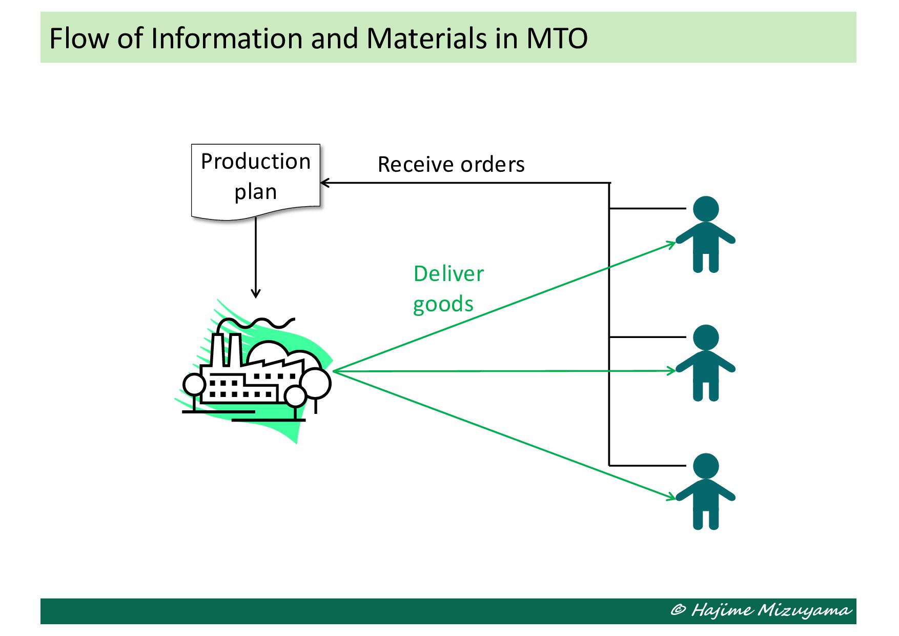
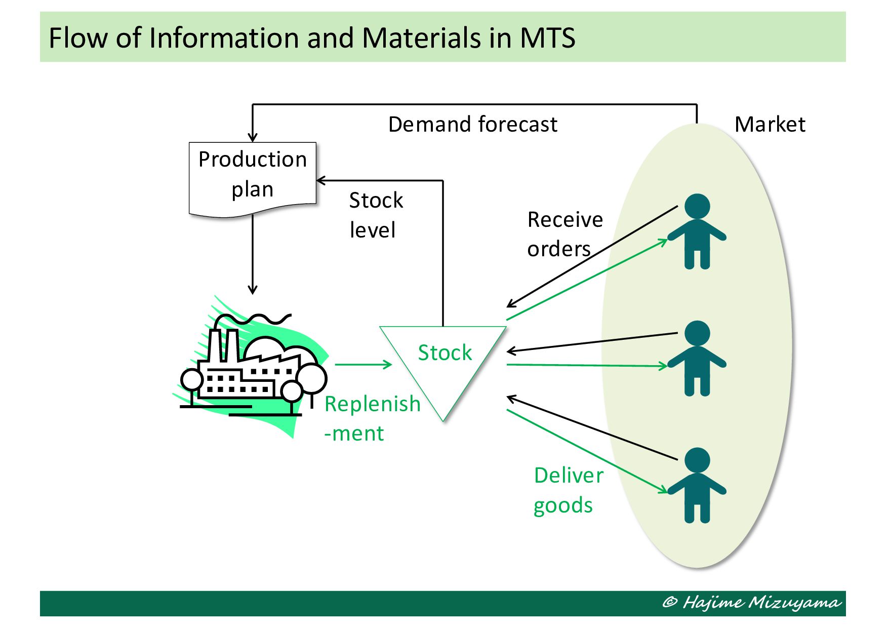
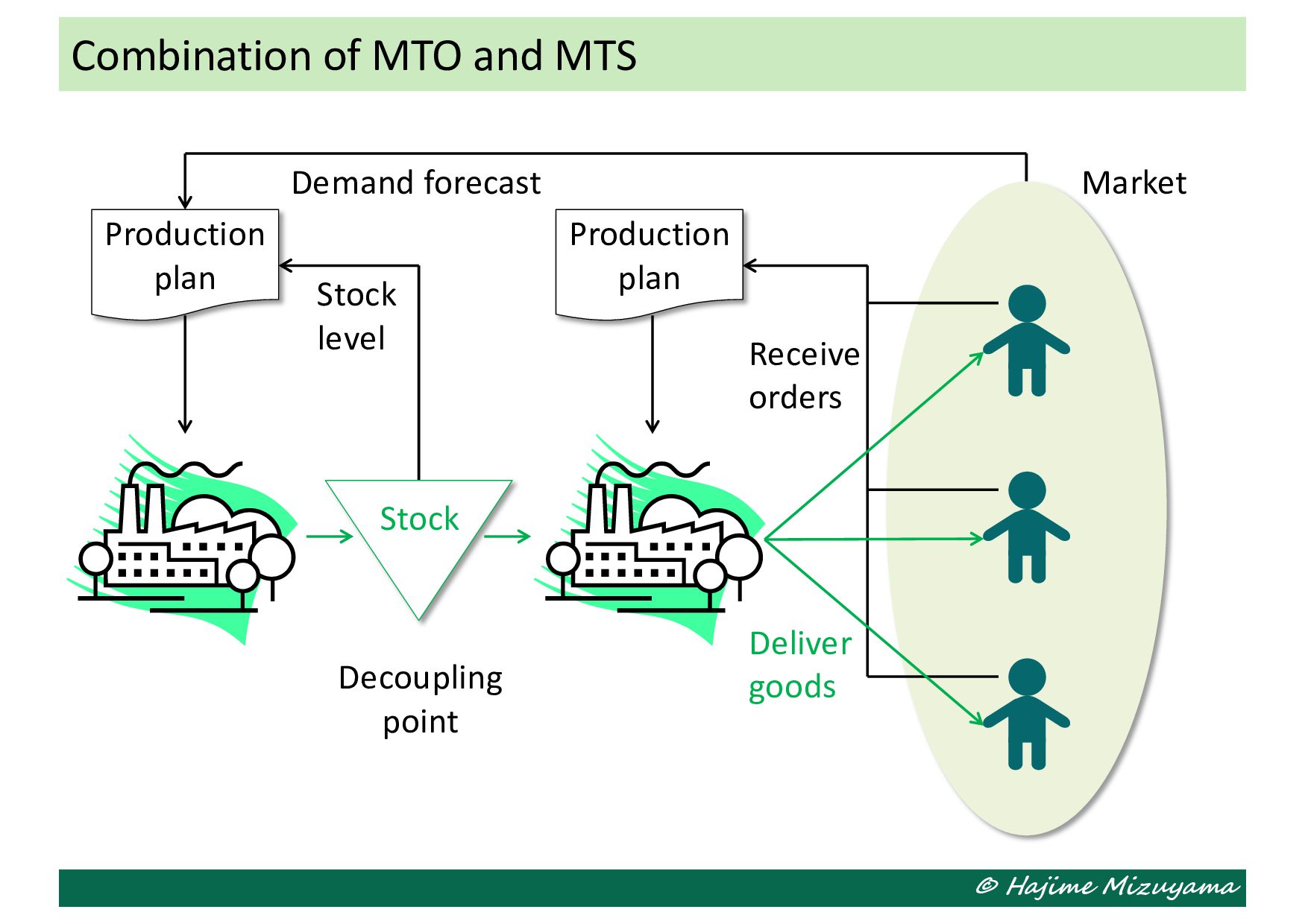
3. © Hajime Mizuyama Make-to-stock: MTS • Products are produced and replenished to the inventory, then they are sold to customers from the inventory. Make-to-order: MTO • After receiving orders from customers, the products corresponding to the orders are produced. These policies can be combined. For example, it is often the case that final products are assembled in MTO, but their units and parts are produced in MTS. Classification of Production Systems #4
4. © Hajime Mizuyama Flow of Information and Materials in MTO Production plan Receive orders Deliver goods
5. © Hajime Mizuyama Market Flow of Information and Materials in MTS Receive orders Deliver goods Stock Replenish -ment Production plan Demand forecast Stock level
6. © Hajime Mizuyama Production plan Demand forecast Stock level Market Combination of MTO and MTS Production plan Receive orders Stock Decoupling point Deliver goods
7. © Hajime Mizuyama Order entry MTS Order entry MTO Demand Forecasting and Production Planning Time axis Due date Production lead time
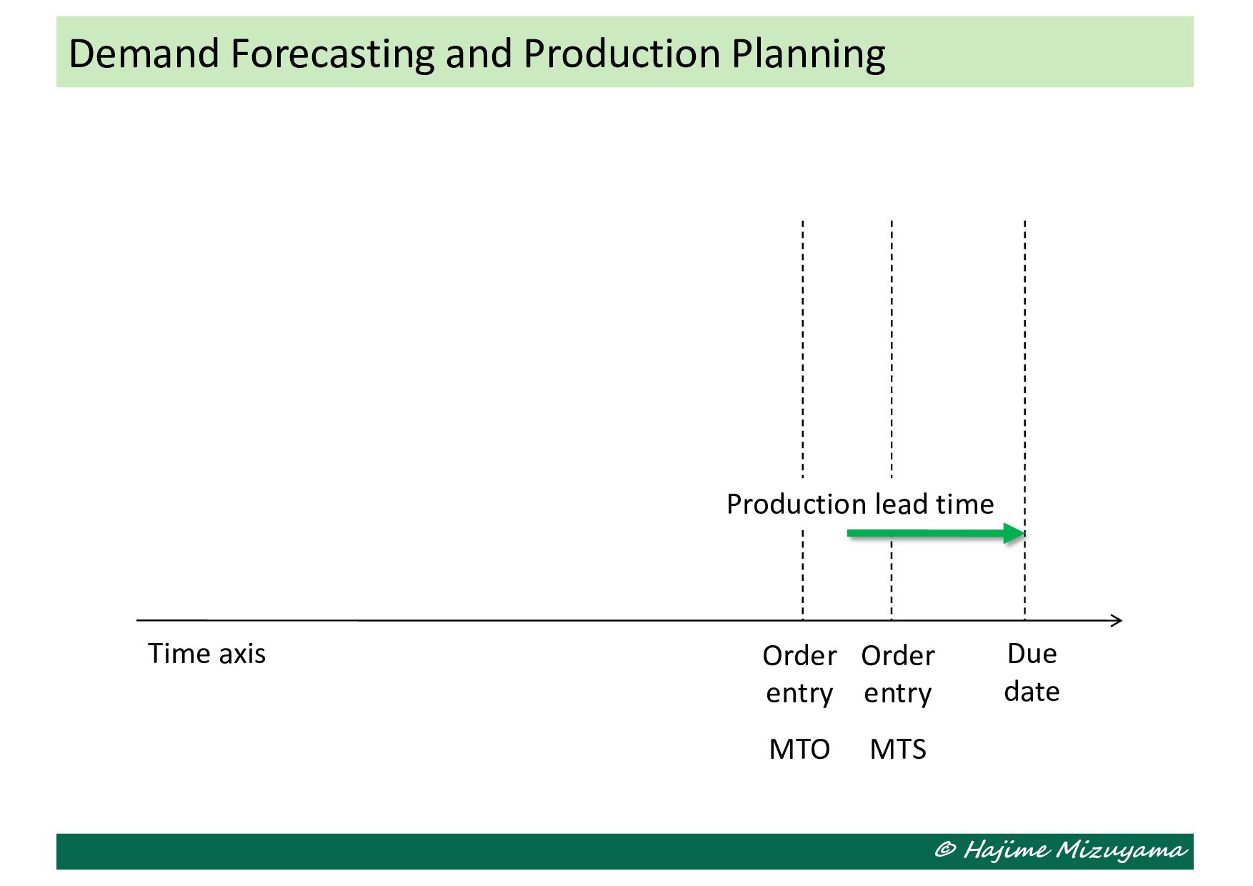
8. © Hajime Mizuyama Order entry MTS Order entry MTO Demand Forecasting and Production Planning Time axis Due date Production lead time 3Ms for production Materials huMans Machines Preparation lead time Necessary means of production should be prepared systematically in advance according to demand forecast not only in MTS but also in MTO production.
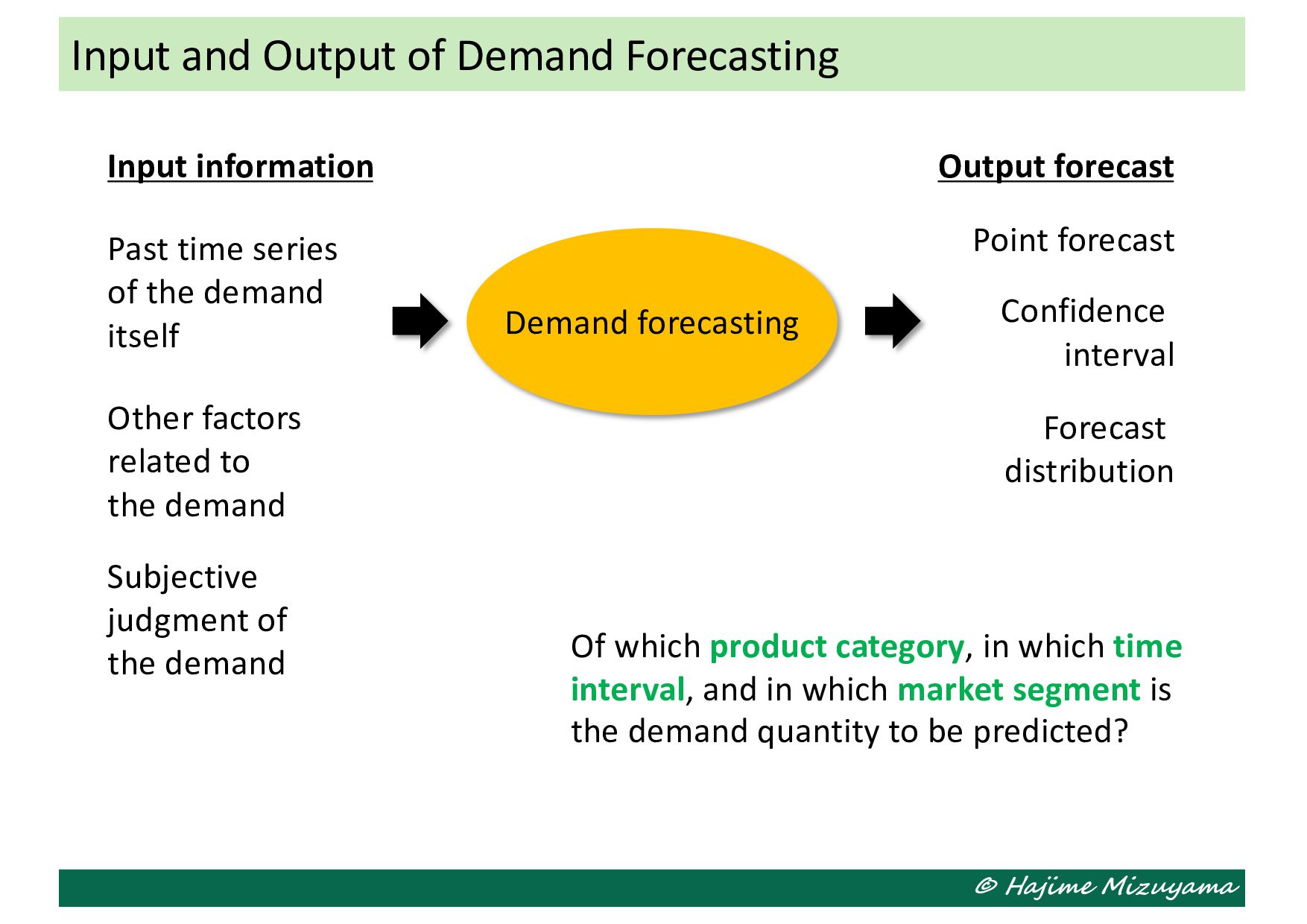
9. © Hajime Mizuyama Demand • The desire to purchase a product. In economics, it is the amount of the product that consumers are willing to buy at a particular price. Demand forecasting • Predict the demand quantity for a product in a future time period. Why necessary? • As a basis for establishing long-term, medium-term, and short-term plans for production and sales. Demand and Demand Forecasting
10. © Hajime Mizuyama Input and Output of Demand Forecasting Demand forecasting Input information Past time series of the demand itself Other factors related to the demand Subjective judgment of the demand Output forecast Point forecast Confidence interval Forecast distribution Of which product category, in which time interval, and in which market segment is the demand quantity to be predicted?
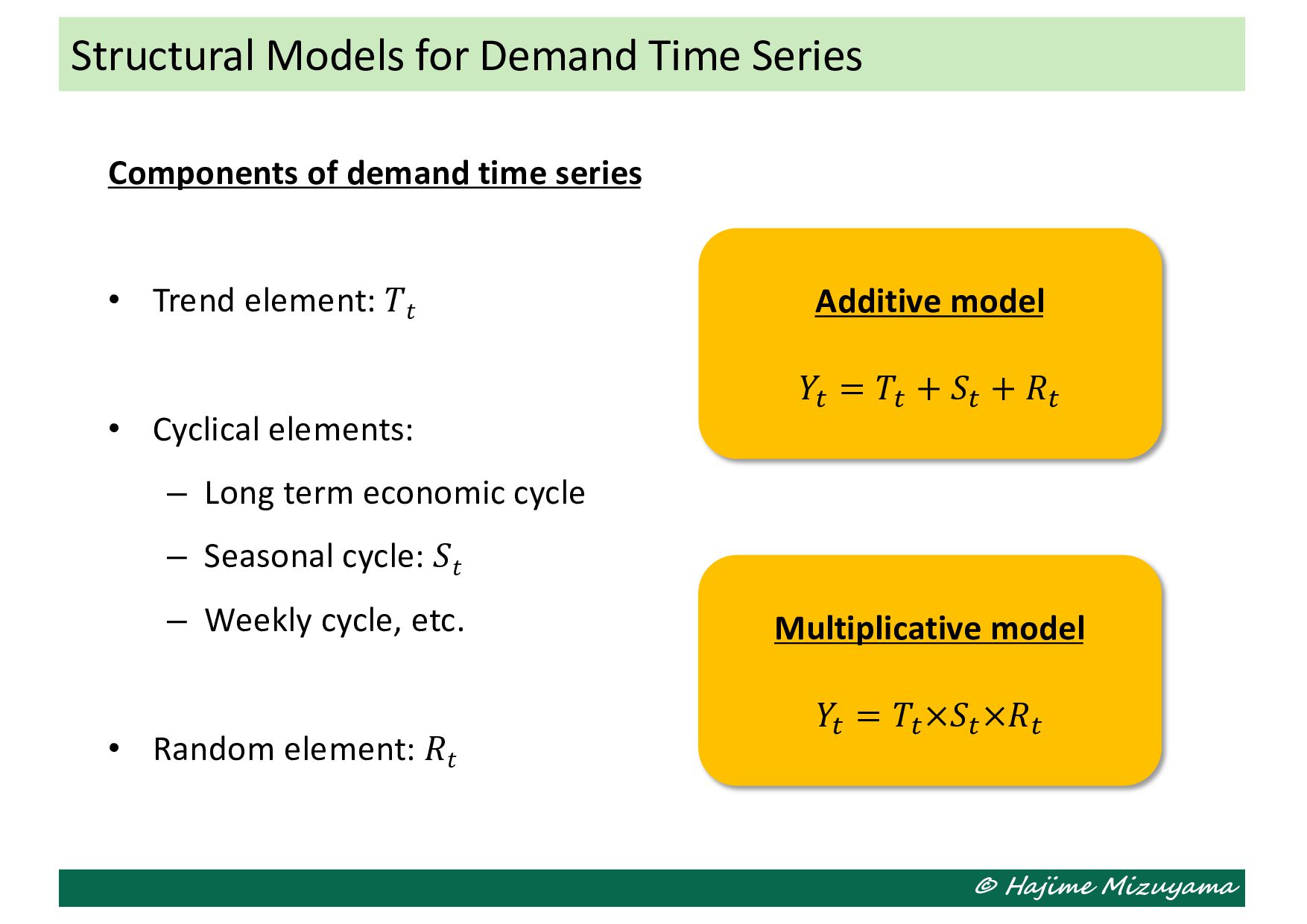
11. © Hajime Mizuyama Components of demand time series • Trend element: 𝑇𝑡 • Cyclical elements: – Long term economic cycle – Seasonal cycle: 𝑆𝑡 – Weekly cycle, etc. • Random element: 𝑅𝑡 Structural Models for Demand Time Series Additive model 𝑌! = 𝑇! + 𝑆! + 𝑅! Multiplicative model 𝑌! = 𝑇! ×𝑆! ×𝑅!
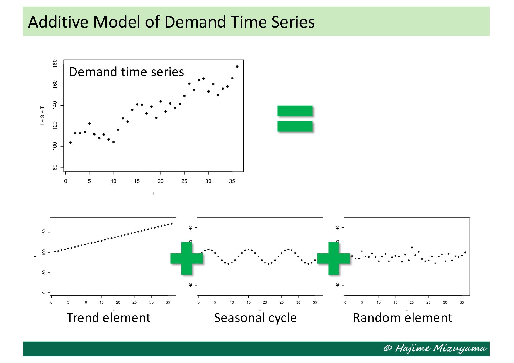
12. © Hajime Mizuyama Additive Model of Demand Time Series 0 5 10 15 20 25 30 35 80 100 120 140 160 180 t I + S + T Demand time series 0 5 10 15 20 25 30 35 0 50 100 150 t T 0 5 10 15 20 25 30 35 -40 -20 0 20 40 t S 0 5 10 15 20 25 30 35 -40 -20 0 20 40 t I Trend element Seasonal cycle Random element
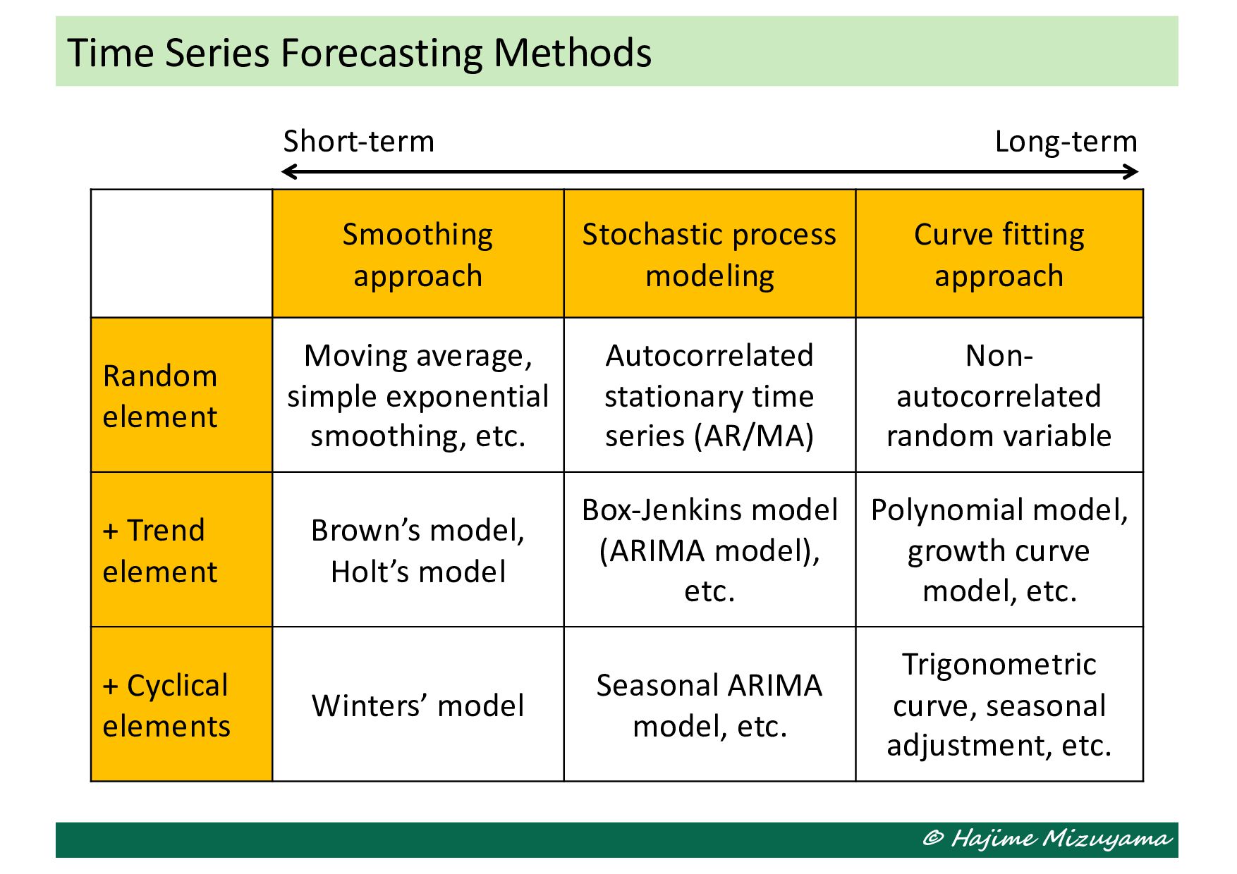
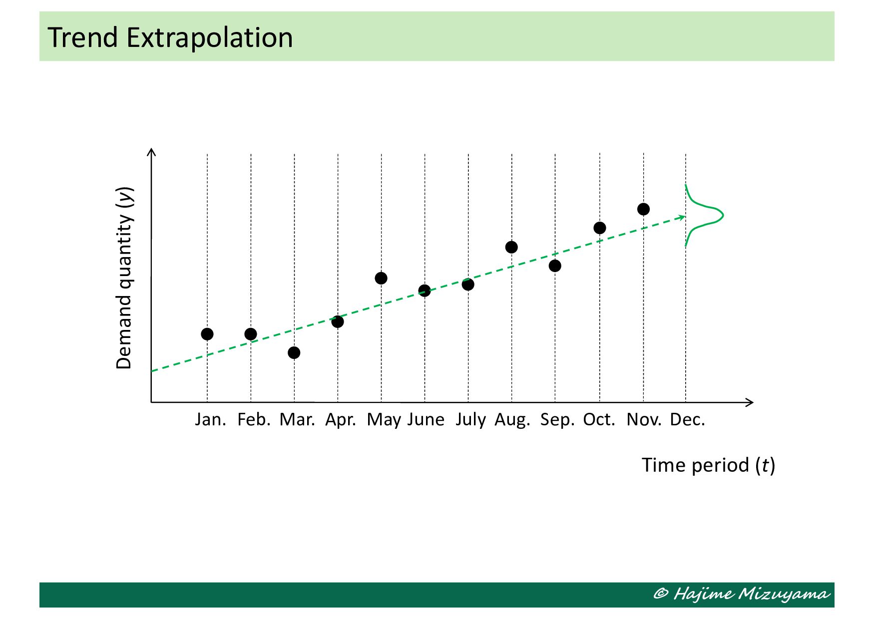
13. © Hajime Mizuyama Smoothing approach Stochastic process modeling Curve fitting approach Random element Moving average, simple exponential smoothing, etc. Autocorrelated stationary time series (AR/MA) Non- autocorrelated random variable + Trend element Brown’s model, Holt’s model Box-Jenkins model (ARIMA model), etc. Polynomial model, growth curve model, etc. + Cyclical elements Winters’ model Seasonal ARIMA model, etc. Trigonometric curve, seasonal adjustment, etc. Time Series Forecasting Methods Short-term Long-term
14. © Hajime Mizuyama Trend Extrapolation Sep. Aug. July June May Apr. Mar. Feb. Jan. Dec. Nov. Oct. Demand quantity (y) Time period (t)
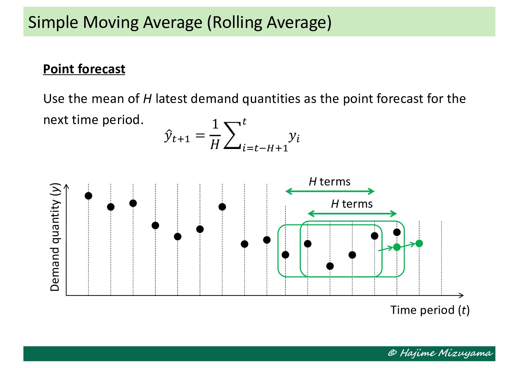
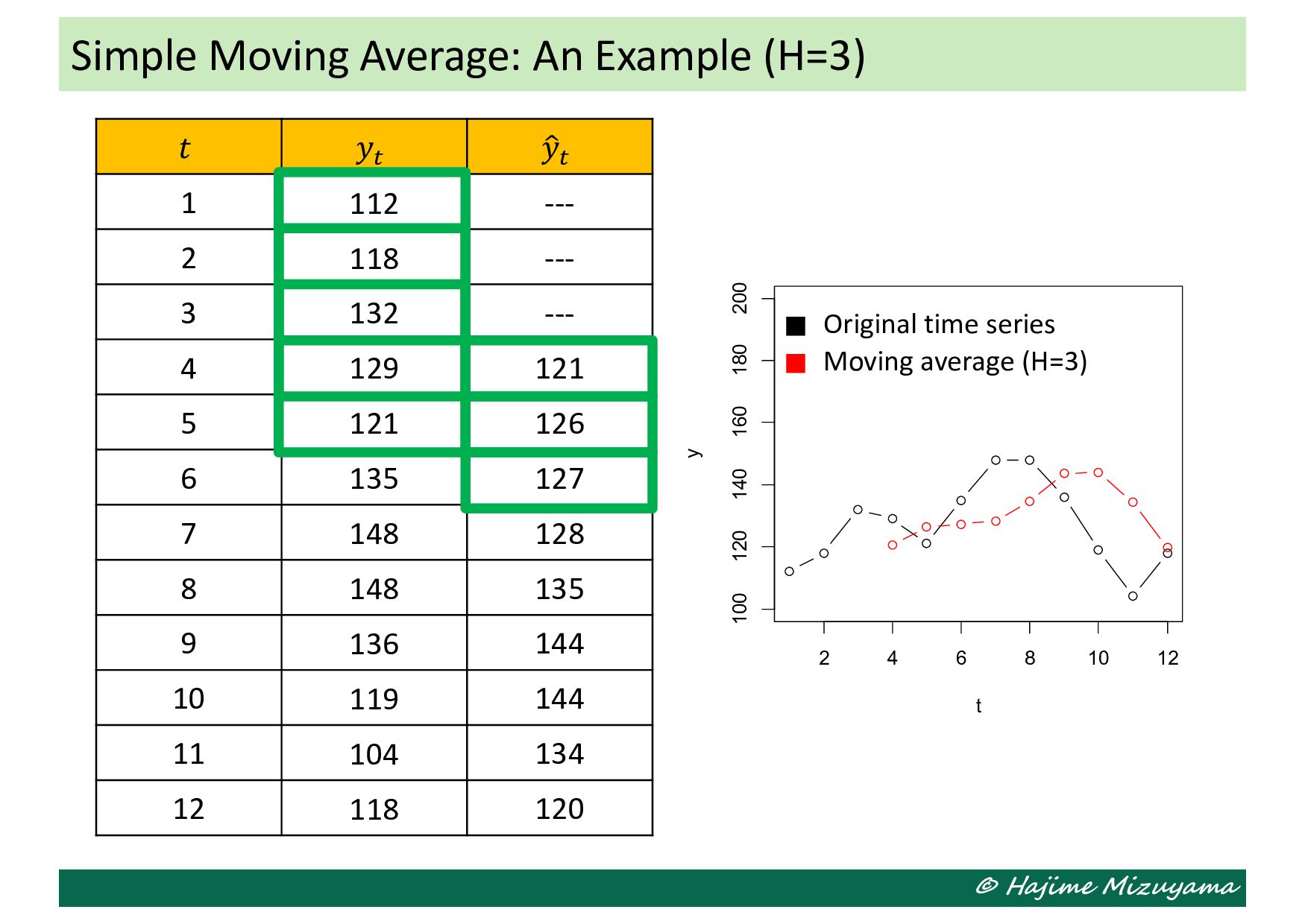
15. © Hajime Mizuyama Point forecast Use the mean of H latest demand quantities as the point forecast for the next time period. Simple Moving Average (Rolling Average) Demand quantity (y) H terms Time period (t) H terms ( 𝑦!"# = 1 𝐻 , $%!&'"# ! 𝑦$
16. © Hajime Mizuyama 𝑡 𝑦! # 𝑦! 1 112 --- 2 118 --- 3 132 --- 4 129 121 5 121 126 6 135 127 7 148 128 8 148 135 9 136 144 10 119 144 11 104 134 12 118 120 Simple Moving Average: An Example (H=3) 2 4 6 8 10 12 100 120 140 160 180 200 t y Original time series Moving average (H=3)
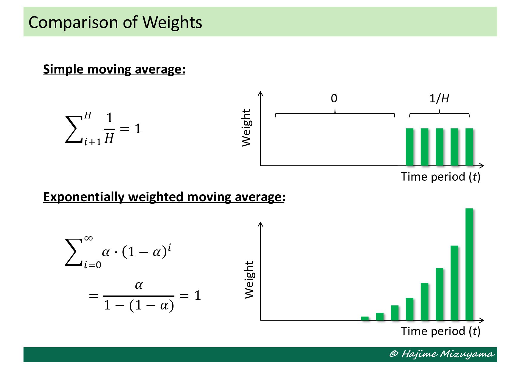
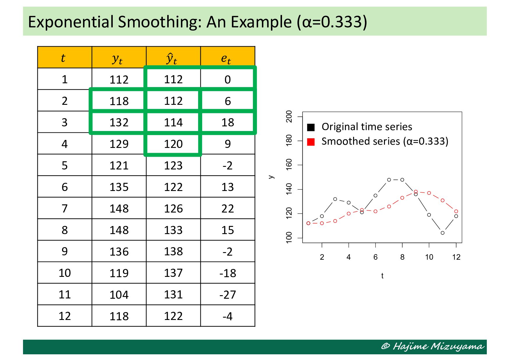
17. © Hajime Mizuyama Point forecast Construct the point forecast for the next time period by combining the forecast value and forecasting error for this period as: ( 𝑦!"# = ( 𝑦! + 𝛼 . 𝑒! = ( 𝑦! + 𝛼 . (𝑦! − ( 𝑦! ) = 𝛼 . 𝑦! + 1 − 𝛼 . ( 𝑦! = ∑$%( ) 𝛼 . 1 − 𝛼 $ . 𝑦$ This is also called exponentially weighted moving average, because of the last expression of the above equation. Exponential Smoothing Weight Time period (t) Smoothing coefficient: 0 < 𝛼 ≤ 1
18. © Hajime Mizuyama Simple moving average: Exponentially weighted moving average: Comparison of Weights Weight Weight 1/H 0 Time period (t) Time period (t) , $"# ' 1 𝐻 = 1 , $%( ) 𝛼 . 1 − 𝛼 $ = 𝛼 1 − (1 − 𝛼) = 1
19. © Hajime Mizuyama 𝑡 𝑦! # 𝑦! 𝑒! 1 112 112 0 2 118 112 6 3 132 114 18 4 129 120 9 5 121 123 -2 6 135 122 13 7 148 126 22 8 148 133 15 9 136 138 -2 10 119 137 -18 11 104 131 -27 12 118 122 -4 Exponential Smoothing: An Example (α=0.333) 2 4 6 8 10 12 100 120 140 160 180 200 t y Original time series Smoothed series (α=0.333)
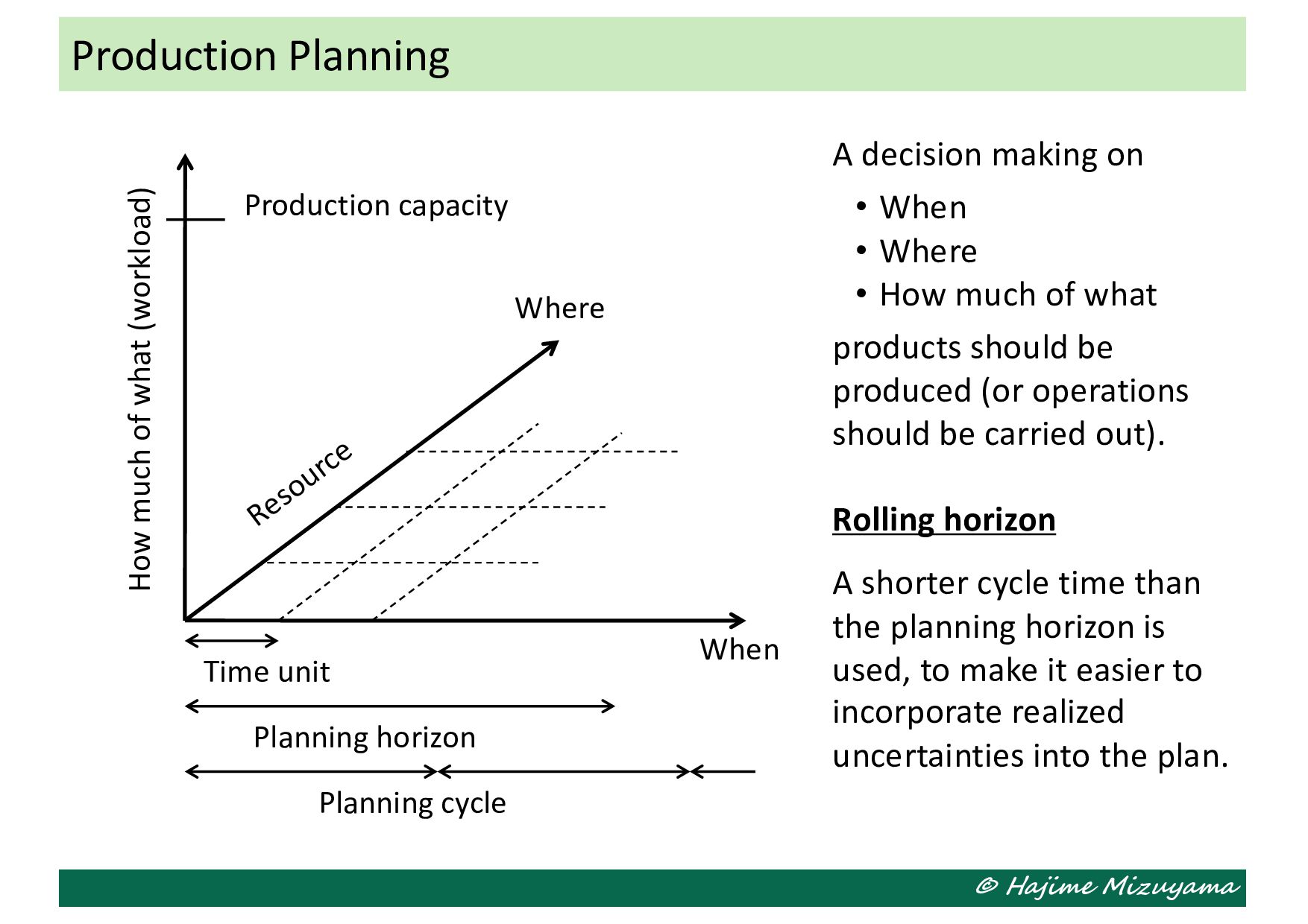
20. © Hajime Mizuyama Production Planning When Where How much of what (workload) Planning horizon Time unit Resource Production capacity Planning cycle A decision making on • When • Where • How much of what products should be produced (or operations should be carried out). Rolling horizon A shorter cycle time than the planning horizon is used, to make it easier to incorporate realized uncertainties into the plan.
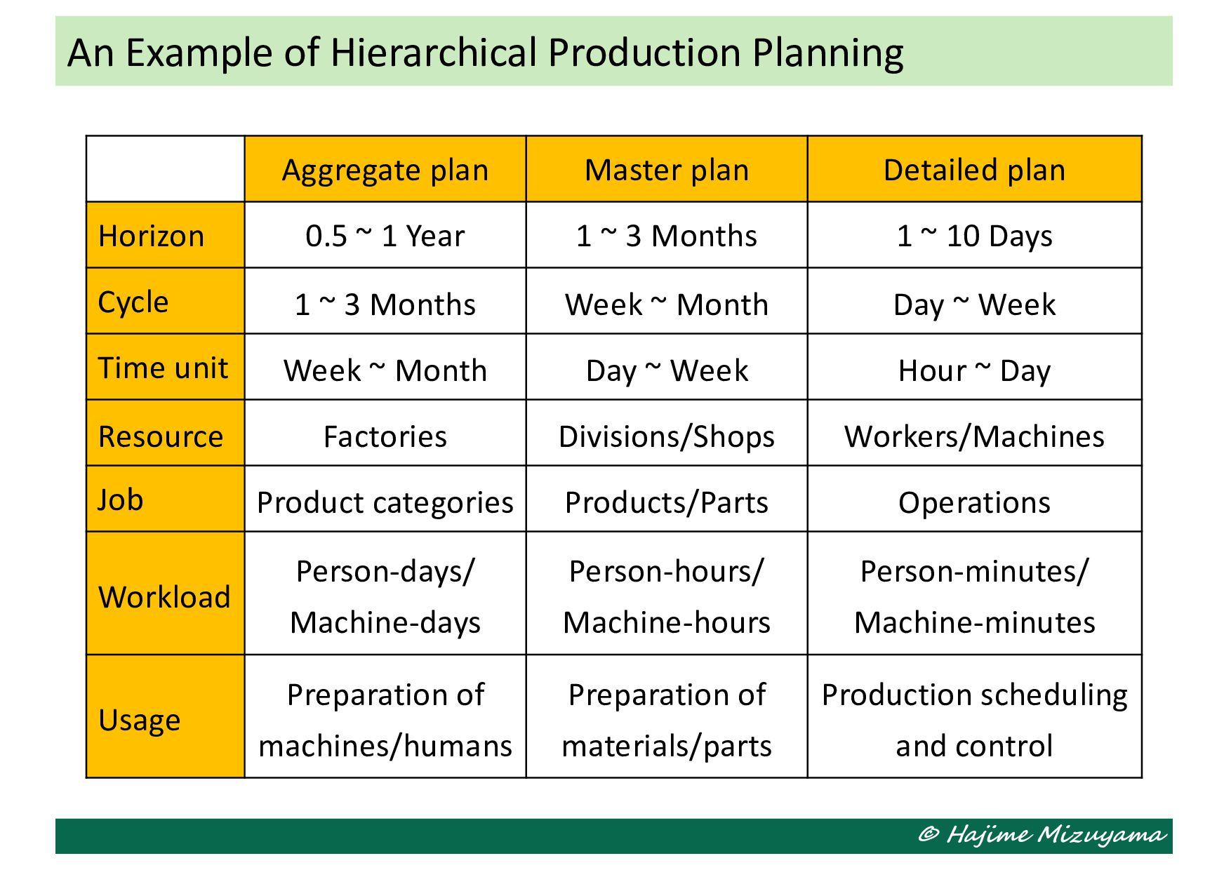
21. © Hajime Mizuyama Aggregate plan Master plan Detailed plan Horizon 0.5 ~ 1 Year 1 ~ 3 Months 1 ~ 10 Days Cycle 1 ~ 3 Months Week ~ Month Day ~ Week Time unit Week ~ Month Day ~ Week Hour ~ Day Resource Factories Divisions/Shops Workers/Machines Job Product categories Products/Parts Operations Workload Person-days/ Machine-days Person-hours/ Machine-hours Person-minutes/ Machine-minutes Usage Preparation of machines/humans Preparation of materials/parts Production scheduling and control An Example of Hierarchical Production Planning
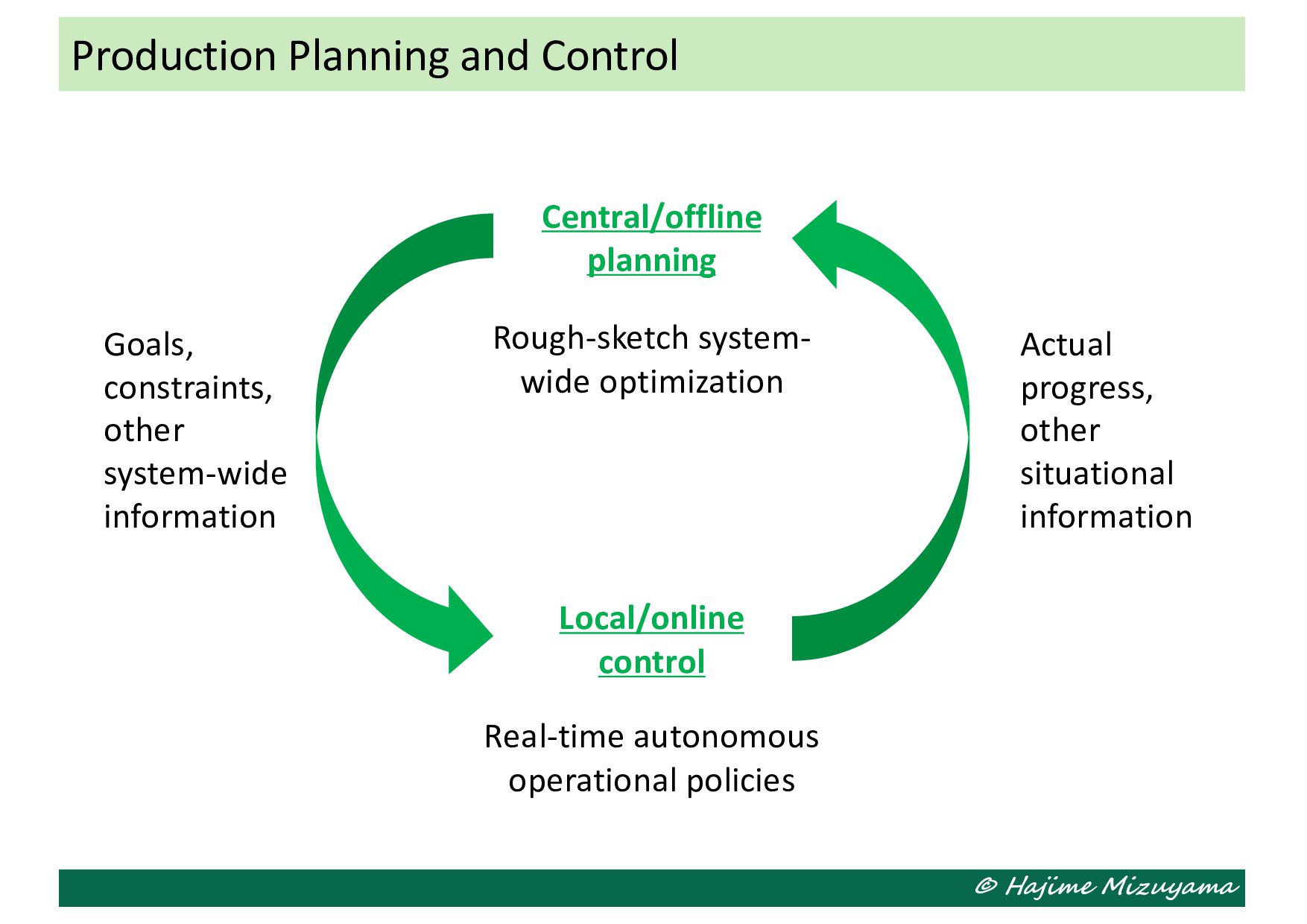
22. © Hajime Mizuyama • Production control is the action of monitoring the difference between the plan and actual progress of production, and taking suitable measures for resolving the gap if necessary. • Since production does not always proceed completely as planned in practice, it needs to be controlled as well as planned appropriately. → Not only P&D but also C&A! • Possible measures include adding resources, rescheduling, and, if necessary, revising production plans of different layers. Production Control
23. © Hajime Mizuyama Production Planning and Control Central/offline planning Local/online control Goals, constraints, other system-wide information Actual progress, other situational information Real-time autonomous operational policies Rough-sketch system- wide optimization