Hyperspectral Analysis of Seagrass in Redfish Bay, Texas

By John S. Wood

Various sources of funding including NOAA ECSC,

Transcript

1. Hyperspectral  Analysis  of  Seagrass  in     Redfish  Bay,  Texas       John  S.  Wood     Various  sources  of  funding  including       NOAA  ECSC,  Center  For  Coastal  Studies,  TPWD,  TGLO       October  3rd,  2012 Texas GIS Forum
2. Acknowledgements       •  CommiQee  Members:    Dr.  James  Gibeaut  and  Dr.  Wes  Tunnell,  Co-­‐Chairs;    Dr.  Gary  Jeffress  (CBI)  and  Dr.  James  Simons  (CCS)   •  NaZonal  Oceanic  and  Atmospheric  AdministraZon      Environmental  CooperaZve  Science  Center  &  Partners   •  UT  Marine  Science  Inst.,  University  of  Nebraska,  Lincoln  (UNL),  TPWD,  CCS   •  Dr.  Larry  McKinney  and  all  the  HRI  Staff   •  Dr.  Elizabeth  Smith,  for  all  the  kind  wishes,  advice  and  encouragement   •  Dr.  Hyun  Jung  ("J.")  Cho,  Bethune-­‐Cookman  University   •  Jennifer  Sweatman,    PhD2B…  
3. Study  Area…  
4. Study  Area   Approximately 3,231 Hectares Depth < 2 m, avg .75 m 5 Types of Seagrass Predominately Halodule wrightii & Thalassia testudinum Located within MANERR Also, Ruppia, Syringodium, Halophila Tidally Influenced Spoil Islands from Dredging Bottom sediment varies, turbidity plumes from channels, boats Aransas  Pass   Rockport   Port    Aransas  
5. MoZvaZon  and  ObjecZve   •  Seagrasses  Are  An   Important  Indicator  Species   •  Monitoring  Is  Important   •  Texas  Seagrass  Monitoring   Program  -­‐  2000   •  In  Decline  Worldwide  (?)   •  Species  Successional   •  Develop  EffecZve  Processing  Methods   Worldwide  Seagrass  DistribuZon   Schull  2005   •  Coastal  &  Marine  SpaZal  Planning  
6. Other  methods   •  Swim  Surveys  -­‐  Manual    Mapping   •  Analog  Imagery,  Photography   •    Velum  or  DigiZze   •  MulZspectral  Digital  Imagery   •  object  oriented   •  simply  not  enough  info  
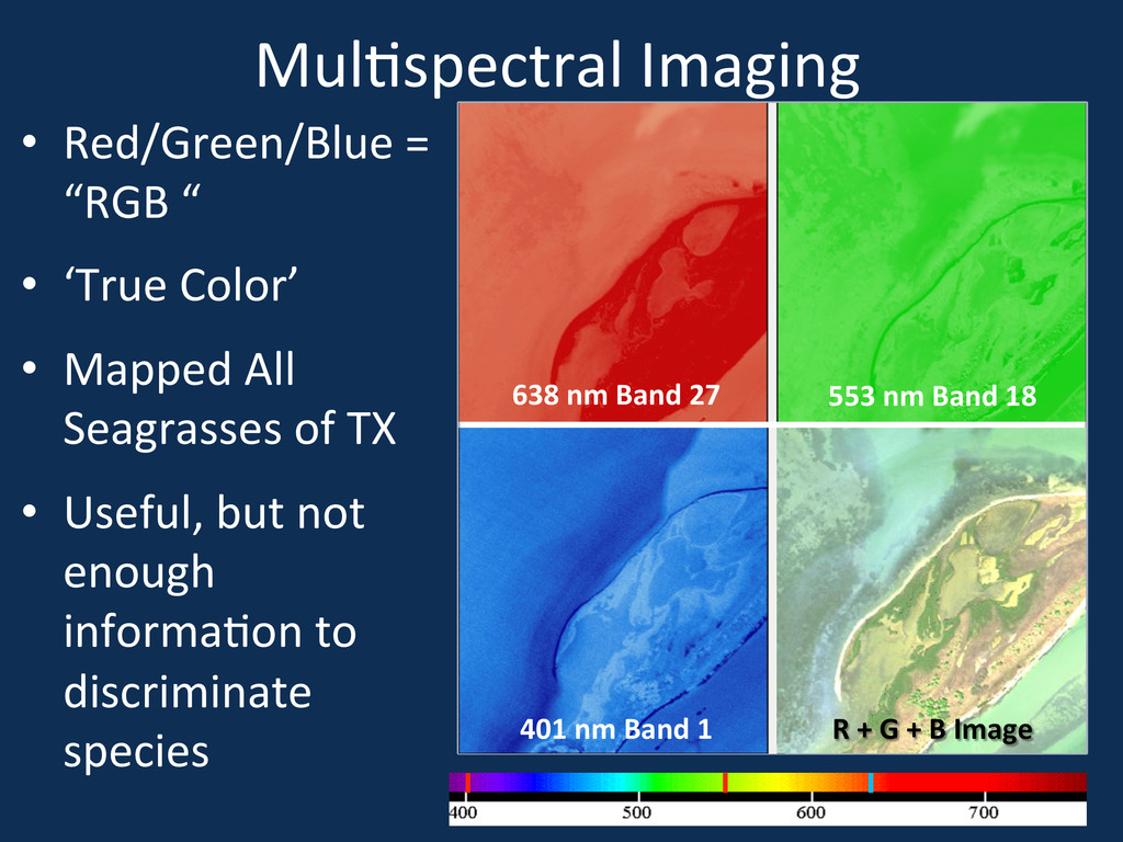
7. •  Red/Green/Blue  =       “RGB  “   •  ‘True  Color’   •  Mapped  All   Seagrasses  of  TX   •  Useful,  but  not   enough   informaZon  to   discriminate   species   MulZspectral  Imaging   401  nm  Band  1   553  nm  Band  18   638  nm  Band  27   R  +  G  +  B  Image  
8. What  is     ‘Hyperspectral  Imagery’?   Adapted  from  Shull  (2000)   hQp://www.yorku.ca/eye/toc.htm  
9. •  Numerous  bands   •  Adjustable,  from  6-­‐8   to  as  many  as  242   bands   •  This  image  shows  56   of  the  63  bands   available  from  the   AISA  Eagle  imagery     used  in  this  research  
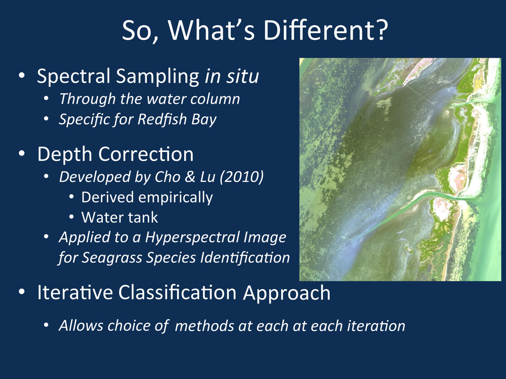
10. So,  What’s  Different?   •  Spectral  Sampling  in  situ   •  Through  the  water  column   •  Specific  for  Redfish  Bay   •  Depth  CorrecZon     •  Developed  by  Cho  &  Lu  (2010)   •  Derived  empirically   •  Water  tank     •  Applied  to  a  Hyperspectral  Image   for  Seagrass  Species  IdenHficaHon   •  IteraZve  ClassificaZon   •  Allows  choice  of   methods  at  each  at  each  iteraHon Approach  
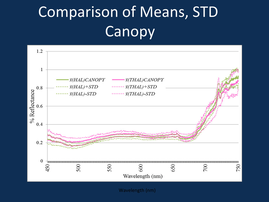
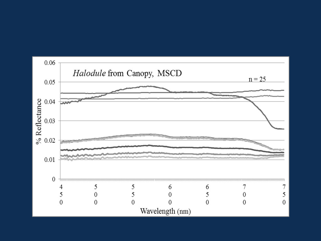
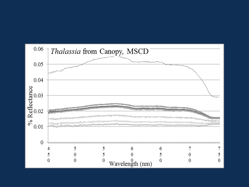
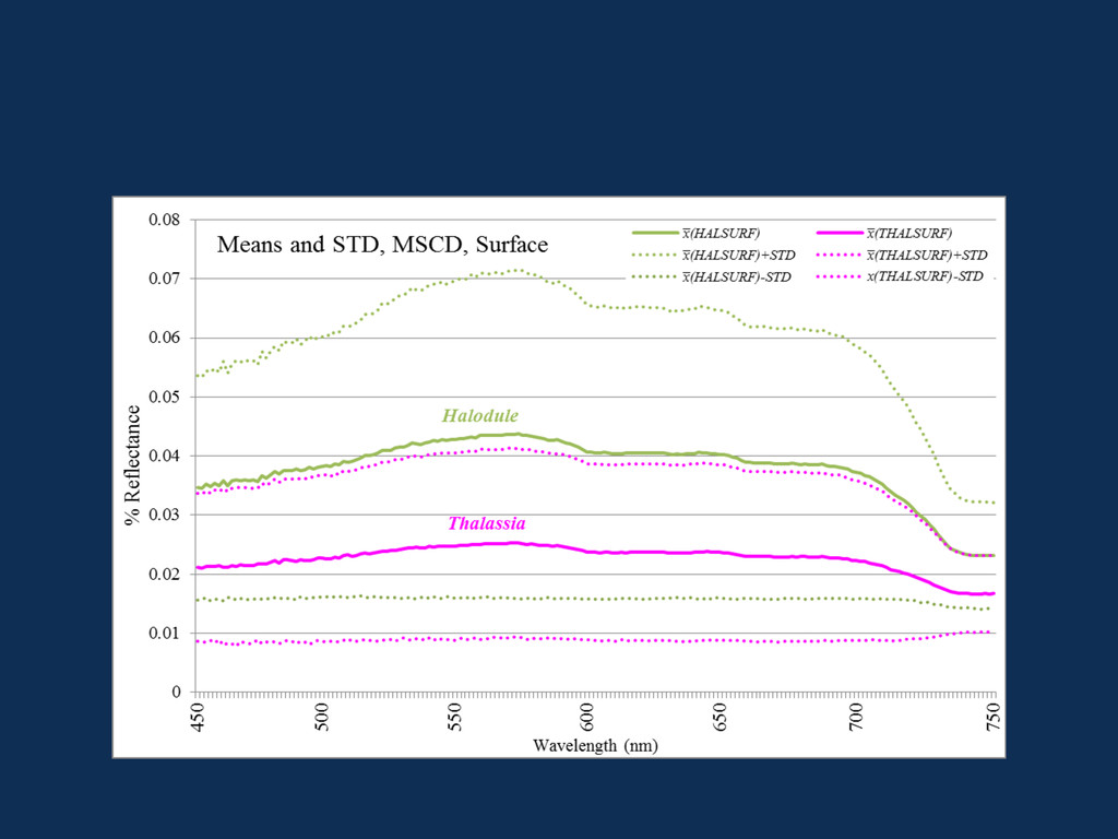
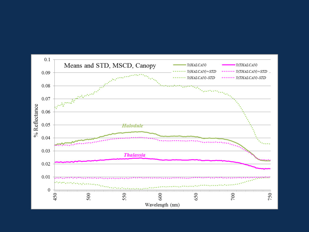
11. Methods   To  Determine  the  Best  Bands   for  Species  DiscriminaGon   •  Collect  Spectral  Signatures   •  Compare  Between  Species   •  Find  Areas  Without  Overlap     To  Apply  to  Imagery   •  Prepare  Imagery   •  Develop  Process   •  Assess  Results   Photo  Courtesy  Jennifer    Sweatman   Photo  Courtesy  TPWD  
12. Seagrass  Species   Photo  Courtesy  Jennifer    Sweatman   Halodule  wrigh.i   Lots  of  Macroalgal  Shading   Thalassia  testudinum   Photo  Courtesy  Jennifer    Sweatman   Scale  1:500   Scale  1:500  
13. Spectral  Signature  Gathering   Spectral   sampling  at   three  posiZons   •  Surface   •  Subsurface   •  Canopy      
14. FuncZon  for  Depth   CorrecZon  Coefficients     (R λ + 14 – Rwλ ) / (1- Awλ /200)2 ( Cho et al. 2010) Rwλ : Scattering within the Water Column Awλ : Absorption within the Water Column Water  AbsorpGon   and  ScaMer   Awλ Rwλ Rwλ
15. DistribuZon  of  Samples  by  Depth   Count   Depth  (cm)  
16. Single  Collected  Spectrum  
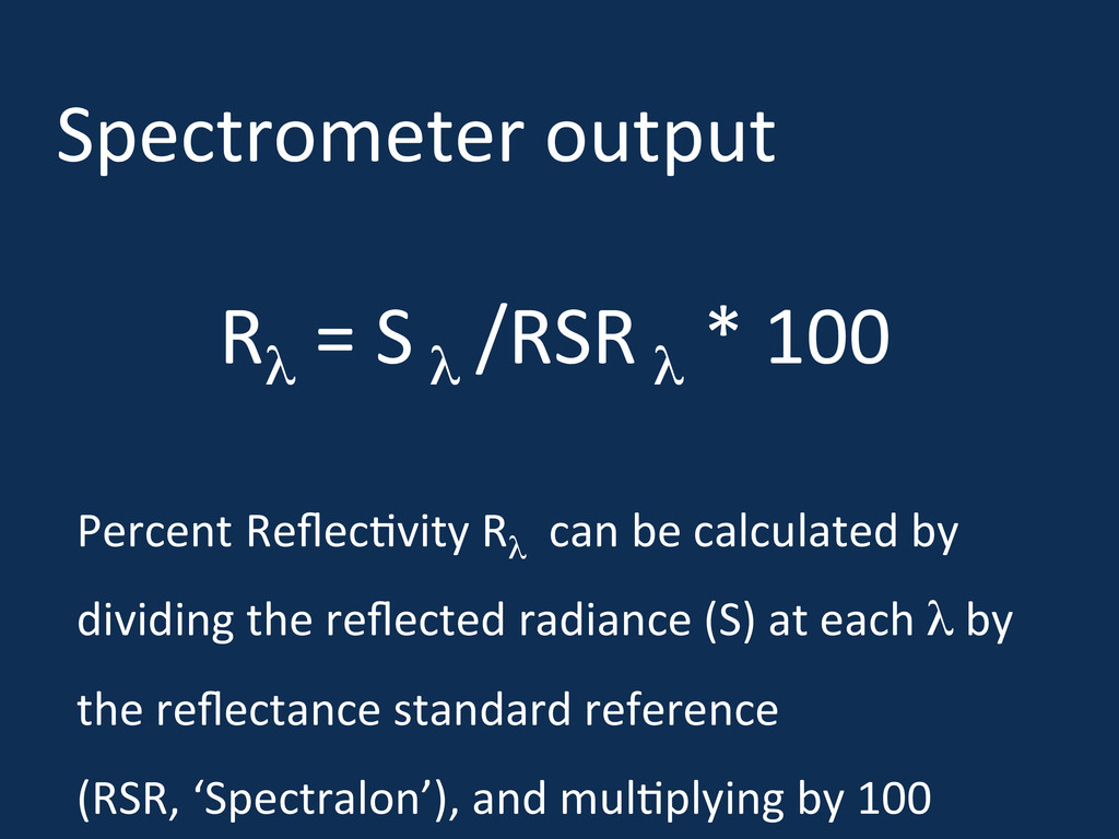
17. Spectrometer  output     Rλ  =  S λ /RSR λ  *  100   Percent ReflecZvity  Rλ    can  be  calculated  by   dividing  the  reflected  radiance  (S)  at  each  λ  by   the  reflectance  standard  reference     (RSR,  ‘Spectralon’),  and  mulZplying  by  100  
18. FuncZon  for  Depth  CorrecZon  Coefficients   •  Values  for  5,  10,  17,  22,  32,  37,  42  cm   •  Volumetric  ScaQering   •  Water  AbsorpZon   (R  +  14  –  Rw )  /  (1-­‐  Aw /200)^2   (cm) AbsorpZon    CorrecZon  Coefficient   (cm) ScaQering  CorrecZon  Coefficient  
19. Comparison  of  Means,  STD  
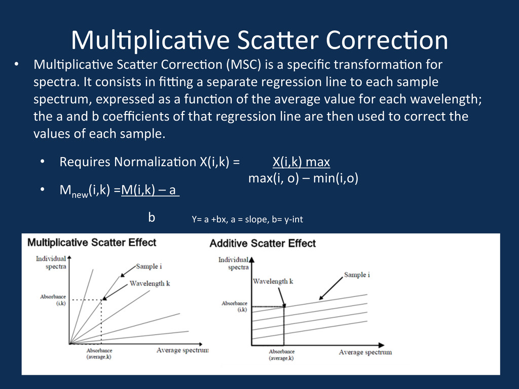
20. MulZplicaZve  ScaQer  CorrecZon   •  MulZplicaZve  ScaQer  CorrecZon  (MSC)  is  a  specific  transformaZon  for   spectra.  It  consists  in  fiung  a  separate  regression  line  to  each  sample   spectrum,  expressed  as  a  funcZon  of  the  average  value  for  each  wavelength;   the  a  and  b  coefficients  of  that  regression  line  are  then  used  to  correct  the   values  of  each  sample.   •  Requires  NormalizaZon  X(i,k)  =                    X(i,k)  max   •  Mnew (i,k)  =M(i,k)  –  a               b   max(i,  o)  –  min(i,o)   Y=  a  +bx,  a  =  slope,  b=  y-­‐int  
21. The  Effects  of   MSCD  and   NormalizaZon  
22. n = 42 The  Effects  of   MSC  and   NormalizaZon  
23. Wavelength  (nm)   Comparison  of  Means,  STD   Canopy  
24. Comparison  of  Means,  STD   Subsurface  
25. Comparison  of  Means,  STD   Surface  
26. Band  SelecZons   % REFLECTANCE, NORM MSC
27. Analysis     Historical – Fyfe 2001 •  5 bands, approximately 5 -10 nm wide each •  500, 555, 635, 650, 675 nm (Fyfe 2001) •  Based on in situ measurements – grass at surface (Fyfe  2001)  
28. Analysis     With Depth Corrections – Cho 2010 •  5 bands, approximately 9-10 nm wide each •  553, 694, 722, 741, 808 nm (personal communications - Cho 2010) •  Achieved 27% Overall Accuracy (Cho  2010)  
29. Analysis     With Depth Correction – Wood 2012 •  5 bands, approximately 9-10 nm wide each •  535, 600, 619, 638, 656 nm (Wood) •  Depth corrections, Band Selection w/ Spectrometer Analysis (Wood  2012)  
30. •  Ground Speed: 120 Knots •  Altitude: 1538.6 m •  Channels: Maximum 240 •  Spatial Resolution: 0.5 – 10 m •  Spectral Resolution: 2.9 nm •  FOV: 39.7º •  IFOV: 0.039º AISA  Eagle   Piper Saratoga Aircraft Airborne Imaging Spectroradiometer for Applications Aerial  Data  CollecZon  
31. Field  work   219 field points collected Summer 2008 ½ (109) used for Signature Development ½ (110) used for Accuracy Assessment 209 Spectral Points Summer 2012
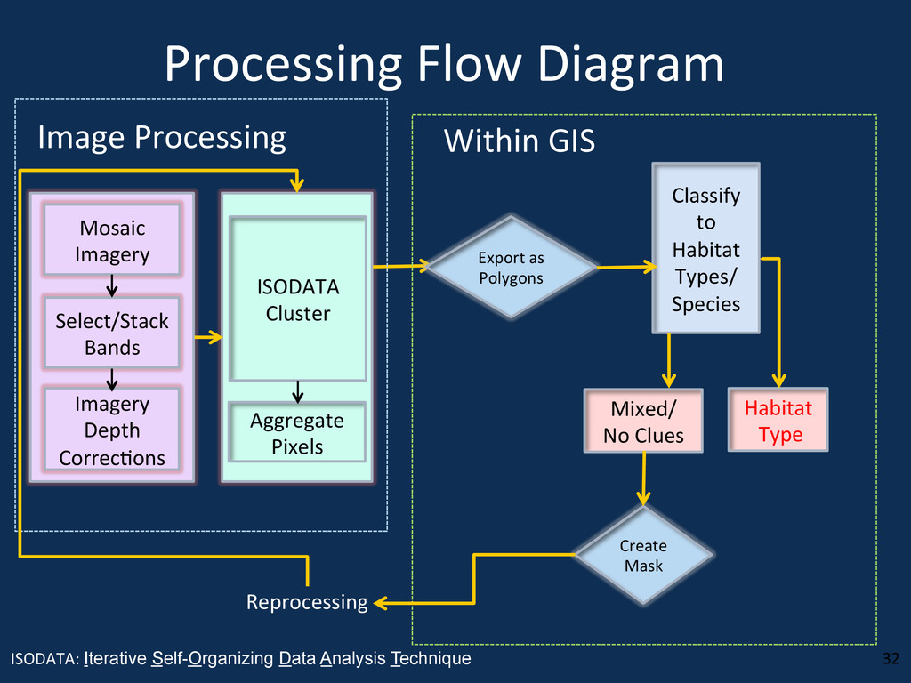
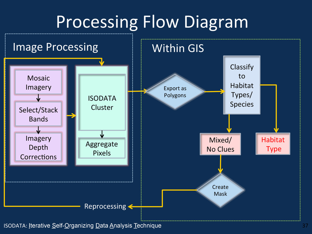
32. Processing  Flow  Diagram   32   ISODATA Cluster   Aggregate Pixels   Select/Stack   Bands   Imagery   Depth   CorrecZons   Mosaic   Imagery   Export  as   Polygons   Classify   to   Habitat   Types/   Species   Mixed/   No  Clues   Habitat    Type   Create   Mask   Within  GIS   Image  Processing     Reprocessing     ISODATA:  Iterative Self-Organizing Data Analysis Technique    
33. Depth  CorrecZons   •  Develop  Bathymetry    Raster     •  Replace  Depth  Values  with     Rw  or  Aw  for  Each  Band (λ)   •  (R  λ +  14  –  Rw λ )  /  (1-­‐  Aw λ /200)2   Rw  λ and  Aw λ  are  Water  ScaQering   and  Water  AbsorpZon  Rasters    
34. First  IteraZon…   CLASS_ NAME AREA MainSpecie grassType Class 1 47 1 H100 Halodule Class 1 150,020 1 H75T25 Mixed Class 1 4,687 * 1 H100, 1 H75T25 Mixed … … … … Class 2 12 * 1 B100, 3 H100, 1 T100, 1 T50S50, 1 H50T50 Mixed … … …
35. Second  IteraZon   •  Mixed  Classes  from   First  IteraZon  as  Mask   •  8,301,542  m2  Classified   •  79,231  Polygons  
36. Third  IteraZon   •  Mixed  Classes  from   Second  IteraZon  as   Mask   •  773,285  m2  Classified   •  Only  27  Polygons  
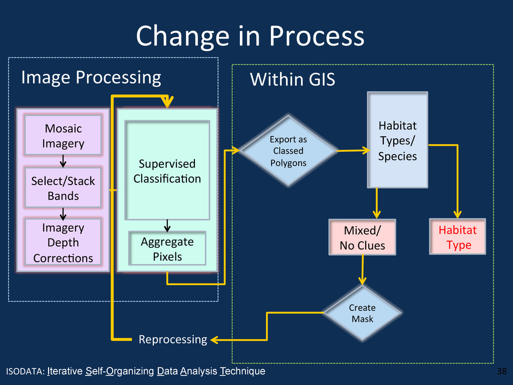
37. Processing  Flow  Diagram   37   ISODATA Cluster   Aggregate Pixels   Select/Stack   Bands   Imagery   Depth   CorrecZons   Mosaic   Imagery   Export  as   Polygons   Classify   to   Habitat   Types/   Species   Mixed/   No  Clues   Habitat    Type   Create   Mask   Within  GIS   Image  Processing     Reprocessing     ISODATA:  Iterative Self-Organizing Data Analysis Technique    
38. Change  in  Process   38   Categorize   Pixels  w/   ISODATA Cluster   Aggregate Pixels   Select/Stack   Bands   Imagery   Depth   CorrecZons   Mosaic   Imagery   Export  as   Polygons   Habitat   Types/   Species   Mixed/   No  Clues   Habitat    Type   Create   Mask   Within  GIS   Image  Processing     Reprocessing     ISODATA:  Iterative Self-Organizing Data Analysis Technique     Export  as   Classed   Polygons   Supervised   ClassificaZon   Aggregate Pixels  
39. Fourth  IteraZon   •  Supervised  ClassificaGon   •  Merged  with  Previous   Output   Mixed 753,857 Halodule 16,805 Bare 1,651 Thalassia 943 Ruppia 29
40. Final  Output   Habitat   m2   Mixed   7,367,203   Halodule   6,125,249   Bare/Halodule  Mix   3,115,812   Thalassia   4,857,068   Bare/Thalassia  Mix   767,466   Bare   4,120,545   Ruppia   462,619   Syringodium   1,042  
41. Areal  Coverage  by  Habitat  Type   Classification   Number of Polygons   Total Area in Class (m2)   Mean Patch Size (m2)   Mixed 38,619 8,063,894 209 Thalassia 22,038 4,976,130 226 Halodule 13,968 3,608,193 258 Ruppia 12,656 3,585,130 283 Bare 2,954 3,537,991 1198 Bare/Thalassia Mix 25,343 3,476,164 137 Bare/Halodule Mix 2,245 587,547 262 Syringodium 2 38,009 19,005 TOTALS 117,825 27,873,058
42. Accuracy  Assessment   Producer’s  Accuracy:    Error  of  omission   Total  number  of  correctly  idenZfied  in  a  class   Total  number  of  reference  data  points  in  a  class   User’s  Accuracy:  errors  of  commission   Total  number  of  correctly  idenZfied  areas  in  a  class   Total  number  of  areas  classified  as  being  that  type   Cohen’s  Kappa:  probability  of  a  chance  agreement   •  Indicates  the  proporZon  of  agreement  beyond  that  expected  by  chance   •  0  è    merely  coincidental,  while  a     •  1  è  no  probability  that  there  is  a  chance  agreement  
43. Accuracy  Assessment   Bare   Halodule   Ruppia   Thalassia   Mixed   Bare   19   3   0   1   3   73%   Halodule   2   24   0   4   6   63%   Ruppia   0   1   0   0   2   0%   Thalassia   3   5   0   12   4   50%   Mixed   3   3   1   4   8   42%   70%   67%   0%   57%   35%   57%   Producer’s  Accuracy    User’s  Accuracy   Bare   73%                Bare   70%         Halodule   63%                Halodule   67%   Ruppia   0%                Ruppia   0%   Thalassia   50%                Thalassia   57%   Mixed   42%                Mixed   35%   Overall  Accuracy                      57%    Kappa  Coefficient                    0.4459    
44. Before  and  Azer   With Depth Correction and New Band Selection Overall Accuracy 57% Cohen's Kappa 0.4459 Without Depth Correction Overall Accuracy 28% With Depth Correction Overall Accuracy 38% Cohen's Kappa 0.2988
45. Presence/Absence   15%   85%   Class Number of Polygons Total Area in Class Bare 2,954 3,537,991 Grass 114,871 24,335,067 TOTALS 117,825 27,873,058 Overall Accuracy 87.93% Cohen’s Kappa .6206
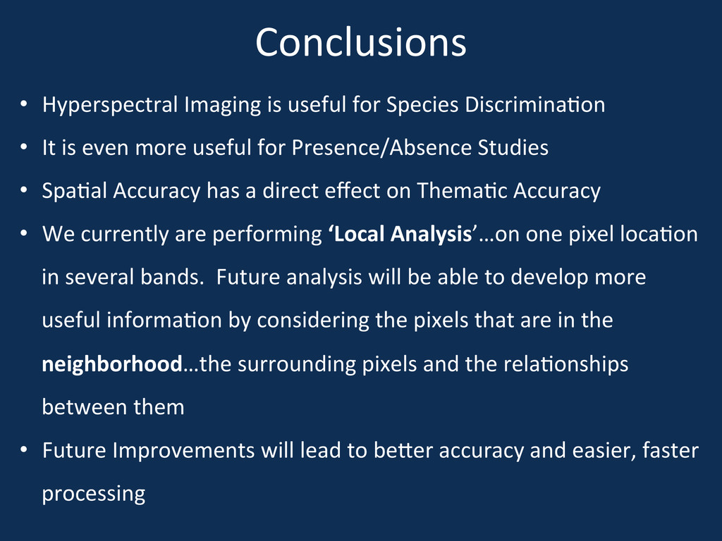
46. Conclusions   •  Hyperspectral  Imaging  is  useful  for  Species  DiscriminaZon   •  It  is  even  more  useful  for  Presence/Absence  Studies   •  SpaZal  Accuracy  has  a  direct  effect  on  ThemaZc  Accuracy   •  We  currently  are  performing  ‘Local  Analysis’…on  one  pixel  locaZon   in  several  bands.    Future  analysis  will  be  able  to  develop  more   useful  informaZon  by  considering  the  pixels  that  are  in  the   neighborhood…the  surrounding  pixels  and  the  relaZonships   between  them   •  Future  Improvements  will  lead  to  beQer  accuracy  and  easier,  faster   processing  
47. QuesZons???   QuesZons?   1)  How  Many  Fish?   2)  What  Type  of  Seagrass?   3)  What’s  All  Over  the  Grass?